<?xml version="1.0" encoding="utf-8"?><feed xmlns="http://www.w3.org/2005/Atom" ><generator uri="https://jekyllrb.com/" version="3.10.0">Jekyll</generator><link href="https://vivekruhela.github.io/archive/feed.xml" rel="self" type="application/atom+xml" /><link href="https://vivekruhela.github.io/archive/" rel="alternate" type="text/html" /><updated>2026-10-15T15:11:48+00:00</updated><id>https://vivekruhela.github.io/archive/feed.xml</id><title type="html">Vivek Ruhela</title><subtitle>Vivek&apos;s academic portfolio</subtitle><author><name>Vivek Ruhela</name><email>vr2592@cumc.columbia.edu</email></author><entry><title type="html">BDL-SP: Using Bio-Inspired Deep Learning to Identify Altered Signaling Pathways in Multiple Myeloma</title><link href="https://vivekruhela.github.io/archive/posts/2026/08/bdl-sp-altered-signaling-pathways-multiple-myeloma/" rel="alternate" type="text/html" title="BDL-SP: Using Bio-Inspired Deep Learning to Identify Altered Signaling Pathways in Multiple Myeloma" /><published>2026-08-19T00:00:00+00:00</published><updated>2026-08-19T00:00:00+00:00</updated><id>https://vivekruhela.github.io/archive/posts/2026/08/BDL-SP%20Altered%20Signaling%20Pathways</id><content type="html" xml:base="https://vivekruhela.github.io/archive/posts/2026/08/bdl-sp-altered-signaling-pathways-multiple-myeloma/"><![CDATA[<h1 id="bdl-sp-using-bio-inspired-deep-learning-to-identify-altered-signaling-pathways-in-multiple-myeloma">BDL-SP: Using Bio-Inspired Deep Learning to Identify Altered Signaling Pathways in Multiple Myeloma</h1>

<p>Multiple myeloma (MM) is a cancer of plasma cells in the bone marrow. It is usually preceded by <strong>monoclonal gammopathy of undetermined significance (MGUS)</strong>, an asymptomatic precursor condition. Most people with MGUS do not rapidly develop MM, yet the two states share many genomic alterations. This makes it difficult to identify which genes and pathways are associated with malignant transformation.</p>

<p>Our study, <strong>“BDL-SP: A Bio-inspired DL model for the identification of altered Signaling Pathways in Multiple Myeloma using WES data,”</strong> introduces an explainable graph-based deep-learning framework for this problem. The work was published in the <em>American Journal of Cancer Research</em> in 2023 (<a href="https://pubmed.ncbi.nlm.nih.gov/37168334/">PubMed</a>; <a href="https://pmc.ncbi.nlm.nih.gov/articles/PMC10164815/">full text in PubMed Central</a>). The associated code and supplementary results are available in the <a href="https://github.com/vivekruhela/BDL-SP-Bio-inspired-DL-architecture-for-Identification-of-altered-Signaling-Pathways-in-MM">BDL-SP GitHub repository</a>.</p>

<p>BDL-SP stands for <strong>Bio-inspired Deep Learning architecture for the identification of altered Signaling Pathways</strong>. Its central premise is that genes do not act independently. They participate in protein-interaction networks and signaling pathways. BDL-SP therefore combines patient-specific genomic measurements with a protein–protein interaction (PPI) graph, then uses post-hoc explainability to connect model predictions back to genes, genomic features, and biological pathways.</p>

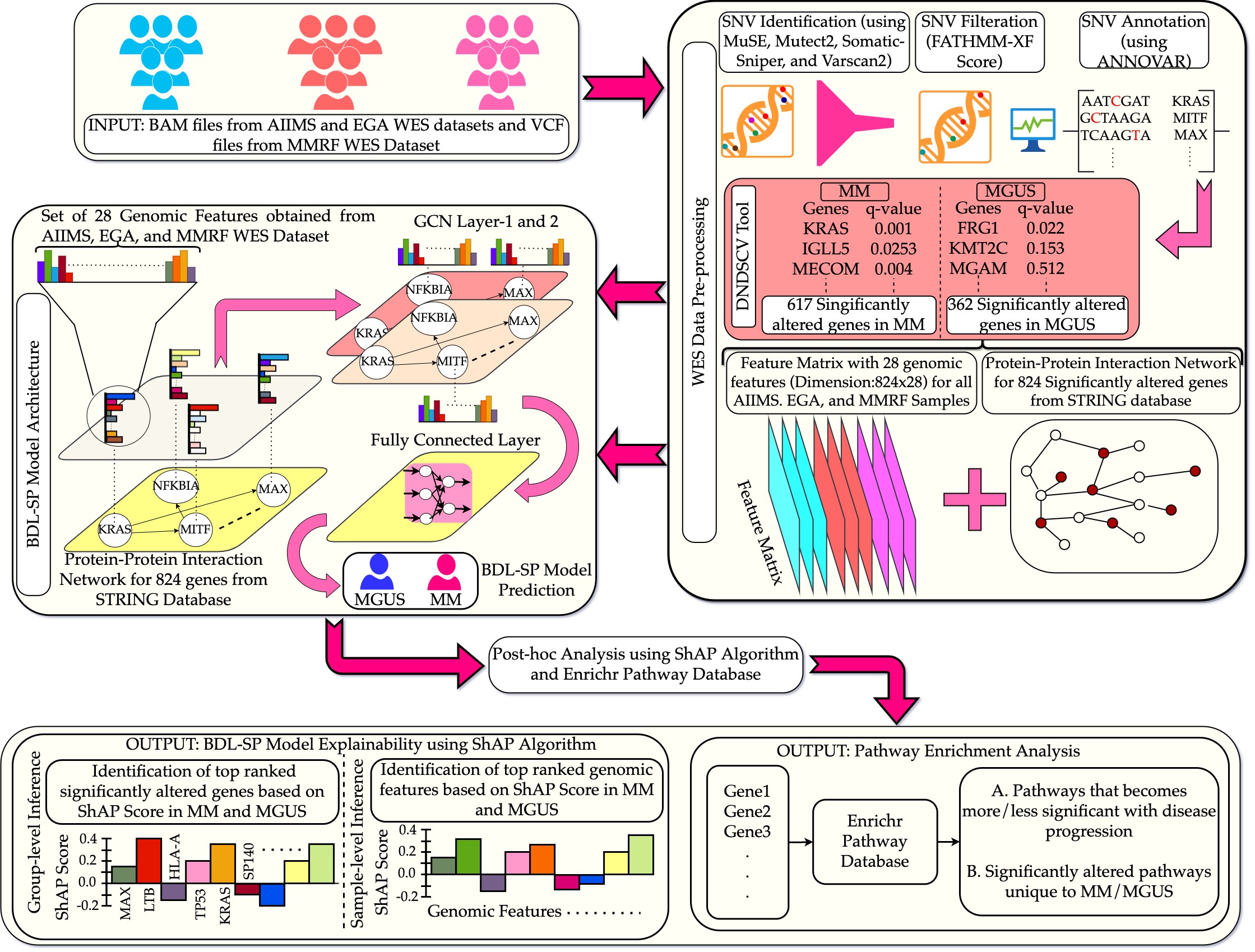
<p><img src="https://raw.githubusercontent.com/vivekruhela/BDL-SP-Bio-inspired-DL-architecture-for-Identification-of-altered-Signaling-Pathways-in-MM/main/figures/bdl-sp-architecture_v6.jpg" alt="BDL-SP workflow showing whole-exome preprocessing, genomic feature extraction, a graph-convolutional model, SHAP interpretation, and pathway analysis" /></p>

<p><em>Figure 1. Overview of the BDL-SP architecture and analysis workflow. Source: <a href="https://github.com/vivekruhela/BDL-SP-Bio-inspired-DL-architecture-for-Identification-of-altered-Signaling-Pathways-in-MM/blob/main/figures/bdl-sp-architecture_v6.jpg">BDL-SP repository</a>.</em></p>

<blockquote>
  <p><strong>In one sentence:</strong> BDL-SP learns from the genomic profiles and known interactions of 824 altered genes, distinguishes MGUS from MM, and uses SHAP and pathway enrichment to explain which molecular signals contributed to the distinction.</p>
</blockquote>

<hr />

<h2 id="background-why-study-the-transition-from-mgus-to-mm">Background: Why study the transition from MGUS to MM?</h2>

<p>MM develops through the accumulation and selection of genomic abnormalities. Some events may already exist during MGUS, whereas others emerge or become more important during progression. Studying these differences can help answer several biological questions:</p>

<ol>
  <li>Which genes are significantly altered in MGUS, MM, or both?</li>
  <li>Which genomic feature types contribute most strongly to separating the two stages?</li>
  <li>Do interacting groups of genes provide more information than isolated mutations?</li>
  <li>Which pathways gain or lose statistical significance as disease advances?</li>
  <li>Can an AI model be interpreted at both the cohort and individual-sample levels?</li>
</ol>

<p>These questions are difficult because MGUS and MM are heterogeneous, the available cohorts are highly imbalanced, and most samples are cross-sectional rather than paired longitudinal specimens from the same people.</p>

<p>BDL-SP was designed as a <strong>biomarker- and pathway-discovery framework</strong>. It is not an approved clinical diagnostic and does not, by itself, predict whether an individual with MGUS will progress to MM.</p>

<hr />

<h2 id="the-study-data">The study data</h2>

<p>The paper analyzed tumor–normal matched whole-exome sequencing (WES) data from three geographic cohorts:</p>

<table>
  <thead>
    <tr>
      <th>Data source</th>
      <th>Population represented</th>
      <th style="text-align: right">Samples used</th>
    </tr>
  </thead>
  <tbody>
    <tr>
      <td>MMRF CoMMpass</td>
      <td>American</td>
      <td style="text-align: right">1,092 MM</td>
    </tr>
    <tr>
      <td>European Genome-phenome Archive</td>
      <td>European</td>
      <td style="text-align: right">33 MGUS</td>
    </tr>
    <tr>
      <td>AIIMS, New Delhi</td>
      <td>Indian</td>
      <td style="text-align: right">82 MM and 28 MGUS</td>
    </tr>
    <tr>
      <td><strong>Total</strong></td>
      <td>Three geographic cohorts</td>
      <td style="text-align: right"><strong>1,174 MM and 61 MGUS</strong></td>
    </tr>
  </tbody>
</table>

<p>This combined design increased cohort size and population coverage, but the MM and MGUS classes remained strongly imbalanced. It also means that disease stage, study source, sequencing workflow, and population background may be partly entangled and must be considered when interpreting the results.</p>

<hr />

<h2 id="from-wes-reads-to-an-explainable-graph-model">From WES reads to an explainable graph model</h2>

<p>The workflow begins with BAM files and proceeds through variant calling, annotation, gene selection, feature construction, graph learning, and interpretation.</p>

<pre><code class="language-mermaid">flowchart TD
    A["Tumor-normal WES BAM files"] --&gt; B["Four somatic variant callers"]
    B --&gt; C["ANNOVAR annotation"]
    C --&gt; D["dNdScv gene analysis"]
    D --&gt; E["824-gene union"]
    E --&gt; F["824 × 28 feature matrix"]
    G["STRING PPI network"] --&gt; H["BDL-SP graph model"]
    F --&gt; H
    H --&gt; I["MGUS versus MM classification"]
    H --&gt; J["SHAP interpretation"]
    J --&gt; K["Gene and pathway ranking"]
</code></pre>

<h3 id="step-1-variant-calling-with-four-tools">Step 1: Variant calling with four tools</h3>

<p>The study used four somatic-variant callers:</p>

<ul>
  <li>MuSE,</li>
  <li>Mutect2,</li>
  <li>SomaticSniper, and</li>
  <li>VarScan2.</li>
</ul>

<p>Using several callers can improve sensitivity to variants detected under different statistical assumptions. However, caller outputs are not interchangeable; reproducible use requires explicit filtering, quality thresholds, genome build, and normalization rules.</p>

<h3 id="step-2-functional-annotation">Step 2: Functional annotation</h3>

<p>Variants were annotated with <strong>ANNOVAR</strong> to connect sequence-level changes with genes and functional categories.</p>

<h3 id="step-3-identification-of-significantly-altered-genes">Step 3: Identification of significantly altered genes</h3>

<p>The workflow used <strong>dNdScv</strong> to identify genes showing evidence of selection. It found:</p>

<ul>
  <li>362 significantly altered genes in MGUS,</li>
  <li>617 significantly altered genes in MM, and</li>
  <li>155 genes shared by both stages.</li>
</ul>

<p>Taking the union produced <strong>824 genes</strong> for model construction. The union strategy was intended to retain stage-specific signals rather than restricting the model to genes common to both conditions.</p>

<h3 id="step-4-construction-of-28-genomic-features">Step 4: Construction of 28 genomic features</h3>

<p>For each of the 824 genes, the workflow generated 28 genomic features. They summarize three broad SNV groups:</p>

<ul>
  <li>non-synonymous SNVs,</li>
  <li>synonymous SNVs, and</li>
  <li>other SNVs, including variants outside those two coding categories.</li>
</ul>

<p>The feature set includes mutation counts and distribution summaries involving measures such as variant allele fraction (VAF) and allele depth (AD). Each patient is therefore represented by a matrix with <strong>824 gene rows and 28 genomic-feature columns</strong>.</p>

<h3 id="step-5-addition-of-biological-structure">Step 5: Addition of biological structure</h3>

<p>The 824 genes were connected using protein-interaction information from <strong>STRING</strong>. This produces an adjacency matrix describing which gene products are connected in the prior interaction network.</p>

<hr />

<h2 id="bdl-sp-model-architecture">BDL-SP Model Architecture</h2>

<p>The released implementation uses a normalized STRING-derived adjacency matrix with self-loops. For every patient, the graph model processes the 824-by-28 feature matrix through two graph-convolution stages.</p>

<p>The repository code documents the following configuration:</p>

<table>
  <thead>
    <tr>
      <th>Component</th>
      <th>Released configuration</th>
    </tr>
  </thead>
  <tbody>
    <tr>
      <td>Input</td>
      <td>824 genes × 28 genomic features</td>
    </tr>
    <tr>
      <td>PPI graph</td>
      <td>STRING-derived adjacency matrix</td>
    </tr>
    <tr>
      <td>Graph layers</td>
      <td>Two graph-convolution layers</td>
    </tr>
    <tr>
      <td>Hidden dimensions</td>
      <td>28 → 7 → 1 per gene</td>
    </tr>
    <tr>
      <td>Activation</td>
      <td>Leaky ReLU</td>
    </tr>
    <tr>
      <td>Dropout</td>
      <td>0.75</td>
    </tr>
    <tr>
      <td>Output</td>
      <td>Two classes: MM and MGUS</td>
    </tr>
    <tr>
      <td>Loss</td>
      <td>Cost-sensitive cross-entropy</td>
    </tr>
    <tr>
      <td>Class weights in code</td>
      <td>1:20</td>
    </tr>
    <tr>
      <td>Regularization</td>
      <td>L1 penalty plus dropout</td>
    </tr>
    <tr>
      <td>Optimizer</td>
      <td>Adam</td>
    </tr>
    <tr>
      <td>Evaluation</td>
      <td>Stratified five-fold cross-validation</td>
    </tr>
    <tr>
      <td>Explainability</td>
      <td>SHAP at group and sample levels</td>
    </tr>
  </tbody>
</table>

<p>At a high level, each graph-convolution stage performs three operations:</p>

<ol>
  <li>normalize the interaction graph and add self-connections;</li>
  <li>aggregate each gene’s features with information from neighboring genes; and</li>
  <li>apply a learned transformation and nonlinear activation.</li>
</ol>

<p>After the second graph layer, each gene has a one-dimensional learned representation. The 824 gene values are flattened and passed to a final layer that produces MM/MGUS probabilities.</p>

<h3 id="why-cost-sensitive-learning">Why cost-sensitive learning?</h3>

<p>The dataset contains 1,174 MM samples but only 61 MGUS samples. A naïve classifier could obtain high ordinary accuracy by predicting the majority class. BDL-SP therefore assigns greater loss to errors involving the minority class. The repository code uses a 1:20 class-weight ratio, close to the observed imbalance.</p>

<p>This makes <strong>balanced accuracy</strong>, area under the ROC curve, and area under the precision–recall curve more informative than ordinary accuracy alone.</p>

<h3 id="why-five-fold-evaluation">Why five-fold evaluation?</h3>

<p>In stratified five-fold cross-validation, each fold retains approximately the same class proportions. Every sample is used for testing once and training in the other folds. This provides a more stable estimate than a single split, although external validation on a separately collected cohort remains stronger evidence of generalization.</p>

<hr />

<h2 id="model-performance">Model performance</h2>

<p>The paper compared BDL-SP with six cost-sensitive machine-learning models, including Random Forest, CatBoost, XGBoost, logistic regression, support vector classification, and decision trees.</p>

<p>The three strongest reported models were:</p>

<table>
  <thead>
    <tr>
      <th>Model</th>
      <th style="text-align: right">Balanced accuracy</th>
      <th style="text-align: right">AUC</th>
    </tr>
  </thead>
  <tbody>
    <tr>
      <td><strong>BDL-SP</strong></td>
      <td style="text-align: right"><strong>96.26%</strong></td>
      <td style="text-align: right"><strong>0.99</strong></td>
    </tr>
    <tr>
      <td>Cost-sensitive Random Forest</td>
      <td style="text-align: right">95.5%</td>
      <td style="text-align: right">0.99</td>
    </tr>
    <tr>
      <td>Cost-sensitive CatBoost</td>
      <td style="text-align: right">91.3%</td>
      <td style="text-align: right">0.99</td>
    </tr>
  </tbody>
</table>

<p>The important lesson is not that a deep model automatically dominates conventional ML. Random Forest achieved similar predictive performance. The paper argues that BDL-SP’s additional value emerged in its <strong>application-specific interpretation</strong>: the graph architecture and SHAP analysis recovered more previously reported MM-relevant genes among the leading ranks.</p>

<p>Performance estimates should still be read in the context of the small MGUS group, five-fold reuse of one combined dataset, and potential cohort effects.</p>

<hr />

<h2 id="from-classification-to-explanation-with-shap">From classification to explanation with SHAP</h2>

<p>BDL-SP used SHAP to rank both genes and genomic feature types according to their contribution to model predictions.</p>

<h3 id="group-level-interpretation">Group-level interpretation</h3>

<p>At the group level, the analysis ranked all 824 genes across MM and MGUS. The paper reports <strong>KIR3DL2, IGLL5, and FCGR2A</strong> as the three highest-ranked genes by the study’s best-SHAP-score procedure.</p>

<p>Other leading genes included previously reported MM-associated drivers and biomarkers such as:</p>

<ul>
  <li>HLA-A,</li>
  <li>KRAS,</li>
  <li>LTB,</li>
  <li>TP53,</li>
  <li>EGR1,</li>
  <li>FGFR3,</li>
  <li>NFKBIA,</li>
  <li>IRF1, and</li>
  <li>NRAS.</li>
</ul>

<p>The ranked lists also contained oncogenes such as CARD11, NOTCH1, VAV1, IRS1, MGAM, and ABL2; tumor-suppressor genes such as HLA-B, HLA-C, and SDHA; and actionable-gene candidates including KRAS, NOTCH1, TP53, FGFR3, and ARID1B.</p>

<p>Among 31 previously reported oncogenes present in the 824-gene space, BDL-SP placed:</p>

<ul>
  <li>20 in its top 250 genes, and</li>
  <li>27 in its top 500 genes.</li>
</ul>

<p>These recovery counts support biological relevance, but they are not independent validation when prior databases are also used to assess the resulting ranking.</p>

<h3 id="sample-level-interpretation">Sample-level interpretation</h3>

<p>The analysis also generated gene rankings for individual samples. For each patient, SHAP was applied to fold models that correctly predicted the sample, and the contribution with the largest absolute value was used as the “best SHAP score.”</p>

<p>This helps answer a different question from group-level analysis: not “Which genes matter on average?” but “Which genomic attributes most influenced this particular prediction?”</p>

<p>Sample-level explanations are useful for studying heterogeneity, but they can be unstable across model seeds, correlated inputs, and background datasets. Stability analysis is therefore essential before interpreting a rank as patient-specific biology.</p>

<h3 id="ranking-the-28-genomic-features">Ranking the 28 genomic features</h3>

<p>The top three genomic features reported by the paper were:</p>

<ol>
  <li>total number of SNVs,</li>
  <li>total number of SNVs in the “Other SNV” group, and</li>
  <li>standard deviation of VAF among variants in the “Other SNV” group.</li>
</ol>

<p>The finding that synonymous and non-canonical SNV summaries contributed to classification is biologically interesting because it moves attention beyond protein-changing mutations alone. It does not establish that synonymous variants are causal; these signals may reflect regulatory effects, mutation processes, linkage, sequencing properties, or broader genomic instability.</p>

<hr />

<h2 id="connecting-genes-to-altered-signaling-pathways">Connecting genes to altered signaling pathways</h2>

<p>The top 500 BDL-SP-ranked genes were subjected to enrichment analysis using KEGG and Reactome. The study organized pathways into four disease-stage patterns:</p>

<table>
  <thead>
    <tr>
      <th>Category</th>
      <th>Interpretation</th>
    </tr>
  </thead>
  <tbody>
    <tr>
      <td>1</td>
      <td>Significant in both stages but more significant in MM</td>
    </tr>
    <tr>
      <td>2</td>
      <td>Significant in both stages but less significant in MM</td>
    </tr>
    <tr>
      <td>3</td>
      <td>Significant only in MM</td>
    </tr>
    <tr>
      <td>4</td>
      <td>Significant only in MGUS</td>
    </tr>
  </tbody>
</table>

<p>This is more informative than a single list of enriched pathways because it asks how pathway-level evidence changes between precursor and malignant states.</p>

<p>The paper reported:</p>

<ul>
  <li>5 KEGG and 9 Reactome pathways that gained significance from MGUS to MM;</li>
  <li>108 KEGG pathways observed as significantly altered only in MM; and</li>
  <li>134 Reactome pathways observed as significantly altered only in MM.</li>
</ul>

<p>Some pathways that lost significance during progression were associated with other disease types, whereas many pathways unique to or strengthened in MM reflected cancer-related processes.</p>

<p>Pathway enrichment remains a statistical summary. Results depend on the selected gene set, gene universe, database release, overlapping pathway definitions, and multiple-testing correction. “Significant pathway” should not be interpreted as proof that every pathway component is functionally active in every patient.</p>

<hr />

<h2 id="population-related-observations">Population-related observations</h2>

<p>The study compared the number of known oncogenes, tumor-suppressor genes, oncogene/driver genes, and actionable genes across disease stages and geographic cohorts.</p>

<p>It reported significant differences for several gene groups between MM and MGUS in the combined analysis. Differences were also observed between the Indian and European MGUS cohorts, while the compared Indian and American MM cohorts did not show significant differences across all four groups.</p>

<p>These results motivate ancestry-aware follow-up, but “population effect” cannot be separated cleanly from cohort source, sample handling, sequencing protocol, and disease-stage composition in this study design. Future analyses should include genetic ancestry estimates and harmonized processing rather than using study geography as a proxy for ancestry.</p>

<hr />

<h2 id="why-bdl-sp-is-significant">Why BDL-SP is significant</h2>

<h3 id="1-it-combines-genomic-features-with-biological-networks">1. It combines genomic features with biological networks</h3>

<p>The model does not treat genes as unrelated columns. It uses a PPI graph to structure information flow and represent pathway-level relationships.</p>

<h3 id="2-it-addresses-severe-class-imbalance-explicitly">2. It addresses severe class imbalance explicitly</h3>

<p>Cost-sensitive learning and balanced metrics reduce the risk of mistaking majority-class prediction for useful MGUS/MM discrimination.</p>

<h3 id="3-it-connects-prediction-with-biological-interpretation">3. It connects prediction with biological interpretation</h3>

<p>SHAP is applied to genes and genomic feature types at group and sample levels, then gene rankings are linked to known cancer-gene categories and pathway enrichment.</p>

<h3 id="4-it-studies-pathways-as-changing-disease-stage-signals">4. It studies pathways as changing disease-stage signals</h3>

<p>The four-category pathway framework distinguishes pathways that gain significance, lose significance, or appear stage-specific.</p>

<h3 id="5-it-provides-a-bridge-to-later-network-models">5. It provides a bridge to later network models</h3>

<p>BDL-SP established a static STRING-based GCN and explainability workflow. The later BIO-DGI study extended the broader research direction using attention-based edge weighting and multiple PPI resources to derive a focused 295-gene panel.</p>

<hr />

<h2 id="potential-research-applications">Potential research applications</h2>

<p>BDL-SP can support several research directions:</p>

<ol>
  <li>
    <p><strong>Candidate-biomarker discovery</strong><br />
Prioritize genes for functional experiments or independent cohort validation.</p>
  </li>
  <li>
    <p><strong>Pathway-level comparison of MGUS and MM</strong><br />
Investigate biological processes that become stronger, weaker, or stage specific.</p>
  </li>
  <li>
    <p><strong>Patient-heterogeneity analysis</strong><br />
Compare sample-level SHAP profiles and assess whether recurrent explanatory patterns define molecular subgroups.</p>
  </li>
  <li>
    <p><strong>Longitudinal progression studies</strong><br />
Apply a locked model to serial MGUS, smoldering-MM, and MM specimens.</p>
  </li>
  <li>
    <p><strong>Population-aware genomics</strong><br />
Test whether gene and pathway rankings replicate across ancestries under harmonized sequencing and preprocessing.</p>
  </li>
  <li>
    <p><strong>Functional prioritization</strong><br />
Select influential genes and network neighborhoods for CRISPR, cell-line, organoid, or animal-model experiments.</p>
  </li>
  <li>
    <p><strong>Alternative network experiments</strong><br />
Compare STRING with tissue-specific, pathway-specific, or experimentally measured interaction graphs.</p>
  </li>
  <li>
    <p><strong>Method transfer</strong><br />
Adapt the gene-feature-plus-network design to other precursor-to-malignancy transitions.</p>
  </li>
</ol>

<hr />

<h2 id="bdl-sp-compared-with-related-approaches">BDL-SP compared with related approaches</h2>

<table>
  <thead>
    <tr>
      <th>Approach</th>
      <th>Biological structure</th>
      <th>Main strength</th>
      <th>Main limitation</th>
    </tr>
  </thead>
  <tbody>
    <tr>
      <td>Logistic regression / SVM</td>
      <td>None unless engineered</td>
      <td>Transparent baseline</td>
      <td>Limited nonlinear interaction modeling</td>
    </tr>
    <tr>
      <td>Random Forest / CatBoost</td>
      <td>Implicit feature interactions</td>
      <td>Strong tabular performance</td>
      <td>No explicit gene-network message passing</td>
    </tr>
    <tr>
      <td>BDL-SP</td>
      <td>Static STRING PPI graph</td>
      <td>Graph-aware prediction plus SHAP and pathway analysis</td>
      <td>Relies on one context-independent network</td>
    </tr>
    <tr>
      <td>BIO-DGI</td>
      <td>Attention-weighted graph from nine PPI resources</td>
      <td>Learns relative interaction importance and supports panel construction</td>
      <td>More complex and still dependent on prior-network quality</td>
    </tr>
  </tbody>
</table>

<p>The paper’s benchmarking shows why both quantitative and qualitative assessment matter. Similar AUC values do not imply that models learn equally useful biological representations.</p>

<hr />

<h2 id="exploring-the-bdl-sp-repository">Exploring the BDL-SP repository</h2>

<p>The <a href="https://github.com/vivekruhela/BDL-SP-Bio-inspired-DL-architecture-for-Identification-of-altered-Signaling-Pathways-in-MM">public repository</a> contains the model script, SHAP notebooks, supplementary results, figure, dependency list, and an Apache-2.0 license.</p>

<table>
  <thead>
    <tr>
      <th>Repository area</th>
      <th>Purpose</th>
    </tr>
  </thead>
  <tbody>
    <tr>
      <td><code class="language-plaintext highlighter-rouge">src/bdl-sp-top-feature-extraction.py</code></td>
      <td>GCN training, five-fold evaluation, and model-output generation</td>
    </tr>
    <tr>
      <td><code class="language-plaintext highlighter-rouge">src/Notebooks/BDL_SP_SHAP_Analysis.ipynb</code></td>
      <td>Group-level SHAP analysis</td>
    </tr>
    <tr>
      <td><code class="language-plaintext highlighter-rouge">src/Notebooks/samplewise_shap_analysis.ipynb</code></td>
      <td>Sample-level SHAP analysis</td>
    </tr>
    <tr>
      <td><code class="language-plaintext highlighter-rouge">src/Notebooks/shap_individual_feature_plot.ipynb</code></td>
      <td>Individual-feature visualization</td>
    </tr>
    <tr>
      <td><code class="language-plaintext highlighter-rouge">BDL-SP Model results/</code></td>
      <td>Significant genes, pathways, SHAP rankings, diagrams, and pseudocode supplements</td>
    </tr>
    <tr>
      <td><code class="language-plaintext highlighter-rouge">figures/bdl-sp-architecture_v6.jpg</code></td>
      <td>Graphical workflow and model architecture</td>
    </tr>
    <tr>
      <td><code class="language-plaintext highlighter-rouge">requirements.txt</code></td>
      <td>Partial dependency list</td>
    </tr>
    <tr>
      <td><code class="language-plaintext highlighter-rouge">.github/workflows/python-package.yml</code></td>
      <td>Basic install, lint, and pytest workflow</td>
    </tr>
  </tbody>
</table>

<hr />

<h2 id="take-home-message">Take-home message</h2>

<p>BDL-SP demonstrates how prior biological knowledge can be incorporated into deep learning without abandoning interpretability. Starting from WES data, the workflow integrates four variant callers, dNdScv gene selection, 28 genomic features, and a STRING-derived network to model 824 genes across MGUS and MM.</p>

<p>The model achieved a reported balanced accuracy of 96.26% and an AUC of 0.99, while its strongest contribution was the post-hoc biological analysis: recovery of known MM-relevant genes, sample-level explanations, genomic-feature ranking, and classification of pathways according to how their significance changes across disease stages.</p>

<hr />

<h2 id="resources-and-citation">Resources and citation</h2>

<ul>
  <li>Ruhela V, Jena L, Kaur G, Gupta R, Gupta A. <strong>BDL-SP: A Bio-inspired DL model for the identification of altered Signaling Pathways in Multiple Myeloma using WES data.</strong> <em>American Journal of Cancer Research</em>. 2023;13(4):1155–1187. <a href="https://pubmed.ncbi.nlm.nih.gov/37168334/">PubMed</a> · <a href="https://pmc.ncbi.nlm.nih.gov/articles/PMC10164815/">PubMed Central</a></li>
  <li><a href="https://github.com/vivekruhela/BDL-SP-Bio-inspired-DL-architecture-for-Identification-of-altered-Signaling-Pathways-in-MM">BDL-SP source code and supplementary results</a></li>
  <li><a href="https://github.com/vivekruhela/BDL-SP-Bio-inspired-DL-architecture-for-Identification-of-altered-Signaling-Pathways-in-MM/blob/main/figures/bdl-sp-architecture_v6.jpg">BDL-SP architecture figure</a></li>
</ul>

<h3 id="suggested-repository-citation">Suggested repository citation</h3>

<div class="language-text highlighter-rouge"><div class="highlight"><pre class="highlight"><code>Ruhela V, Jena L, Kaur G, Gupta R, Gupta A. BDL-SP: Bio-inspired deep-learning
architecture for identifying altered signaling pathways in multiple myeloma.
https://github.com/vivekruhela/BDL-SP-Bio-inspired-DL-architecture-for-Identification-of-altered-Signaling-Pathways-in-MM
</code></pre></div></div>]]></content><author><name>Vivek Ruhela</name></author><category term="multiple myeloma" /><category term="MGUS" /><category term="whole-exome sequencing" /><category term="graph convolutional network" /><category term="explainable AI" /><category term="signaling pathways" /><summary type="html"><![CDATA[A beginner-friendly and technical guide to BDL-SP, a graph-based explainable deep-learning framework for distinguishing MGUS from multiple myeloma and identifying altered genes and pathways from whole-exome sequencing data.]]></summary></entry><entry><title type="html">From Genomic Complexity to a 295-Gene Panel: How BIO-DGI Studies Multiple Myeloma Progression</title><link href="https://vivekruhela.github.io/archive/posts/2026/08/bio-dgi-295-gene-panel/" rel="alternate" type="text/html" title="From Genomic Complexity to a 295-Gene Panel: How BIO-DGI Studies Multiple Myeloma Progression" /><published>2026-08-19T00:00:00+00:00</published><updated>2026-08-19T00:00:00+00:00</updated><id>https://vivekruhela.github.io/archive/posts/2026/08/BIO-DGI-295-Gene-Panel</id><content type="html" xml:base="https://vivekruhela.github.io/archive/posts/2026/08/bio-dgi-295-gene-panel/"><![CDATA[<h1 id="from-genomic-complexity-to-a-295-gene-panel">From Genomic Complexity to a 295-Gene Panel</h1>

<h2 id="how-bio-dgi-connects-genomic-variation-gene-networks-and-explainable-ai-in-multiple-myeloma">How BIO-DGI connects genomic variation, gene networks, and explainable AI in multiple myeloma</h2>

<p>Multiple myeloma (MM) is a cancer of antibody-producing plasma cells. It is usually preceded by a clinically silent precursor condition called <strong>monoclonal gammopathy of undetermined significance (MGUS)</strong>. Although MGUS is common and only a subset of cases progresses to active disease, the molecular events that distinguish stable precursor disease from malignant transformation remain difficult to resolve.</p>

<p>Our study, <strong>“A comprehensive targeted panel of 295 genes: Unveiling key disease initiating and transformative biomarkers in multiple myeloma,”</strong> addresses this problem with a biologically informed artificial-intelligence framework called <strong>BIO-DGI</strong>—Bio-Inspired Graph Network Learning-based Gene–Gene Interaction. The work was published in <em>Computers in Biology and Medicine</em> in 2025 (<a href="https://pubmed.ncbi.nlm.nih.gov/40617081/">PubMed</a>; <a href="https://doi.org/10.1016/j.compbiomed.2025.110619">DOI</a>). The accompanying research code and analysis notebooks are available in the <a href="https://github.com/vivekruhela/BIO-DGI">BIO-DGI GitHub repository</a>.</p>

<p>The central idea is simple: a gene should not be studied only as an isolated column in a data table. Genes operate in pathways and molecular networks. BIO-DGI therefore combines patient-level genomic features with prior knowledge of protein–protein interactions, allowing the model to learn not only <strong>which genes matter</strong>, but also <strong>which biological relationships may help distinguish MGUS from MM</strong>.</p>

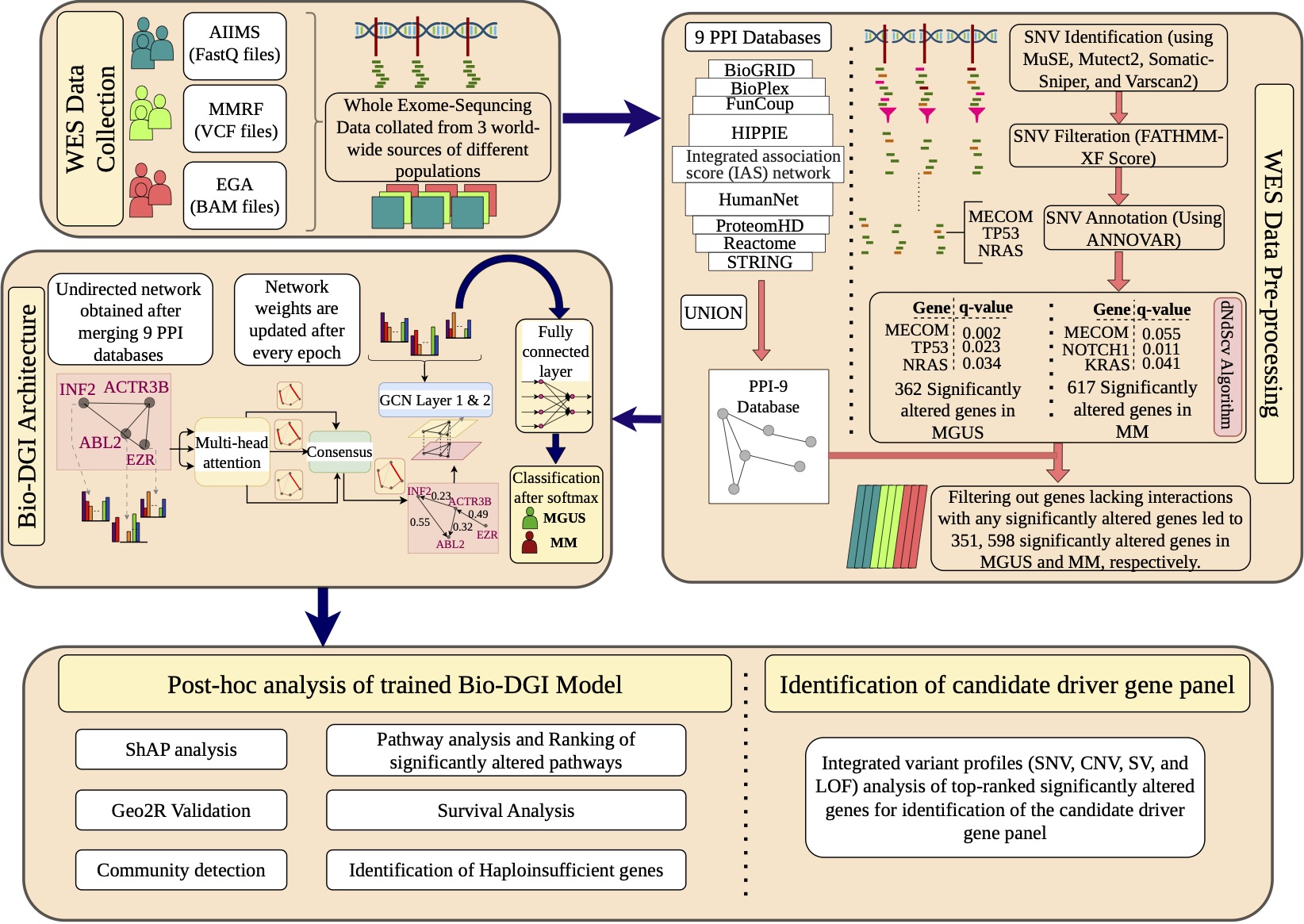
<p><img src="https://raw.githubusercontent.com/vivekruhela/BIO-DGI/main/infographic_abstract.jpg" alt="BIO-DGI graphical abstract showing genomic preprocessing, protein-interaction integration, graph learning, explainability, and panel construction" /></p>

<p><em>Figure 1. Overview of the BIO-DGI workflow. Source: <a href="https://github.com/vivekruhela/BIO-DGI/blob/main/infographic_abstract.jpg">BIO-DGI repository</a>.</em></p>

<blockquote>
  <p><strong>In one sentence:</strong> BIO-DGI treats genes as an interacting biological system, uses explainable graph learning to identify signals separating MGUS from MM, and translates those signals into a focused 295-gene research panel.</p>
</blockquote>

<hr />

<h2 id="background-why-this-problem-matters">Background: Why this problem matters</h2>

<p>MGUS and MM share many genomic alterations. This makes the transition between the two states more subtle than a simple “mutation present versus mutation absent” comparison. Several questions arise:</p>

<ol>
  <li>Which alterations are already present in the precursor state?</li>
  <li>Which genes become selectively altered as malignant disease emerges?</li>
  <li>Do combinations of interacting genes contain more information than single genes considered independently?</li>
  <li>Can a model remain accurate while also providing biologically interpretable evidence?</li>
  <li>Can the resulting discoveries be compressed into a panel that is more practical to investigate than whole-exome or whole-genome sequencing?</li>
</ol>

<p>These questions motivated two useful biological concepts in the paper:</p>

<ul>
  <li><strong>Disease-initiating genes:</strong> genes with alterations detectable in both MGUS and MM, making them candidates for early events in disease development.</li>
  <li><strong>Disease-transformative genes:</strong> genes whose alterations are associated more specifically with the malignant MM state and may help characterize the transition from precursor disease.</li>
</ul>

<p>These labels describe evidence from the analyzed cohorts. They do not, by themselves, prove that an alteration causes disease or that it can predict progression in an individual patient.</p>

<hr />

<h2 id="the-challenge-of-turning-sequencing-data-into-biological-insight">The challenge of turning sequencing data into biological insight</h2>

<p>Whole-exome and whole-genome studies produce high-dimensional data. A single patient can carry many types of genomic change, including:</p>

<ul>
  <li>single-nucleotide variants (SNVs),</li>
  <li>small insertions and deletions,</li>
  <li>copy-number variants (CNVs),</li>
  <li>structural variants (SVs), and</li>
  <li>loss-of-function events.</li>
</ul>

<p>Traditional machine-learning methods often represent every gene as an independent feature. This is convenient, but biologically incomplete. For example, a modest alteration in one gene may become important when several of its interaction partners are also disrupted. Conversely, a frequently altered gene may contribute little to the specific distinction being modeled.</p>

<p>BIO-DGI introduces biological structure before learning begins. Genes are represented as <strong>nodes</strong>, known or predicted protein interactions as <strong>edges</strong>, and genomic measurements as <strong>node features</strong>. The model can then propagate information through the graph and learn which relationships are useful for classifying MM and MGUS profiles.</p>

<pre><code class="language-mermaid">flowchart TD
    A["Patient genomic profiles"] --&gt; B["Gene-level genomic features"]
    C["Nine PPI resources"] --&gt; D["Integrated gene network"]
    B --&gt; E["BIO-DGI graph model"]
    D --&gt; E
    E --&gt; F["MM versus MGUS classification"]
    E --&gt; G["SHAP and network interpretation"]
    G --&gt; H["295-gene research panel"]
</code></pre>

<hr />

<h2 id="study-data-at-a-glance">Study data at a glance</h2>

<p>The study analyzed genomic profiles from <strong>1,154 MM samples</strong> and <strong>61 MGUS samples</strong> collected across American, European, and Indian populations. Starting from sequencing-derived alterations, the workflow identified <strong>798 significantly altered genes</strong> for graph modeling.</p>

<p>For each sample, the repository’s graphical abstract describes <strong>26 genomic features per gene</strong>. These feature vectors summarize multiple aspects of the gene’s alteration profile rather than relying on a single mutation count.</p>

<table>
  <thead>
    <tr>
      <th>Component</th>
      <th>Role in the study</th>
    </tr>
  </thead>
  <tbody>
    <tr>
      <td>1,154 MM profiles</td>
      <td>Represent the malignant disease state</td>
    </tr>
    <tr>
      <td>61 MGUS profiles</td>
      <td>Represent the precursor state</td>
    </tr>
    <tr>
      <td>798 altered genes</td>
      <td>Initial graph nodes considered by BIO-DGI</td>
    </tr>
    <tr>
      <td>26 features per gene</td>
      <td>Patient-specific genomic description of each node</td>
    </tr>
    <tr>
      <td>Nine PPI resources</td>
      <td>Prior knowledge used to construct gene–gene relationships</td>
    </tr>
    <tr>
      <td>295 selected genes</td>
      <td>Final targeted research panel</td>
    </tr>
    <tr>
      <td>9,417 coding regions</td>
      <td>Coding targets covered by the reported panel</td>
    </tr>
    <tr>
      <td>2.630 Mb</td>
      <td>Reported total panel footprint</td>
    </tr>
  </tbody>
</table>

<p>The nine protein-interaction resources integrated in the workflow were <strong>BioGRID, BioPlex, FunCoup, HIPPIE, IAS, HumanNet, ProteomeHD, Reactome, and STRING</strong>. Combining several resources reduces dependence on a single database, although it can also introduce duplicated, predicted, context-independent, or unevenly supported interactions.</p>

<hr />

<h2 id="bio-dgi-model-architecture">BIO-DGI Model Architecture</h2>

<p>For a given patient, the genomic input can be viewed as a feature matrix (X), where rows correspond to genes and columns correspond to genomic measurements. The prior interaction network is represented by an adjacency matrix (A).</p>

<p>BIO-DGI applies a multi-head attention mechanism to learn context-relevant weights for gene–gene relationships. Conceptually, the learned adjacency can be written as:</p>

\[\tilde{A} = \mathrm{Attention}(A,X)\]

<p>A graph-convolutional layer then aggregates each gene’s features with information from its neighbors:</p>

\[H^{(l+1)} = \sigma\!\left(\hat{D}^{-1/2}\hat{A}\hat{D}^{-1/2}H^{(l)}W^{(l)}\right),\]

<p>where (\hat{A}) includes the learned or updated graph structure, (\hat{D}) is its degree matrix, (H^{(l)}) is the representation at layer (l), (W^{(l)}) contains learned parameters, and (\sigma) is a nonlinear activation.</p>

<p>The graph representation passes through a fully connected layer and softmax output for supervised MM-versus-MGUS classification. The essential design choice is that the model does not use a static PPI graph as mere decoration: attention is used to modify the relative importance of edges before graph aggregation.</p>

<h3 id="why-multi-head-attention">Why multi-head attention?</h3>

<p>Different attention heads can learn different relationship patterns. One head might prioritize interactions involving mutation burden, while another could emphasize copy-number or loss-of-function context. The heads do not automatically correspond to clean biological mechanisms, but they increase the capacity to represent more than one interaction pattern.</p>

<h3 id="why-graph-convolution">Why graph convolution?</h3>

<p>Graph convolution encodes the assumption that a gene’s relevance can depend partly on its neighborhood. This is well suited to signaling and protein-interaction systems, where coordinated perturbation may be more informative than isolated events.</p>

<h3 id="why-a-supervised-endpoint">Why a supervised endpoint?</h3>

<p>The MM/MGUS label provides a task-specific learning signal. It directs the network toward patterns that discriminate the malignant and precursor cohorts, after which post-hoc interpretation is used to investigate the model’s biological reasoning.</p>

<hr />

<h2 id="from-prediction-to-explanation">From prediction to explanation</h2>

<p>High classification performance alone is not sufficient for biomarker discovery. A model can exploit technical artifacts, cohort imbalance, or correlates with no mechanistic significance. The study therefore used several complementary interpretation steps.</p>

<h3 id="1-shap-based-feature-interpretation">1. SHAP-based feature interpretation</h3>

<p>SHAP assigns a contribution score to a feature relative to a model prediction. In this setting, it helps answer questions such as:</p>

<ul>
  <li>Which genes contribute most strongly to MM-versus-MGUS discrimination?</li>
  <li>Which genomic feature types drive the importance of a gene?</li>
  <li>Are important signals consistent across samples and model folds?</li>
</ul>

<p>SHAP describes the fitted model; it does not establish causal biology. A high SHAP value means that a feature influenced the model’s prediction under the learned representation.</p>

<h3 id="2-gene-community-analysis">2. Gene-community analysis</h3>

<p>Biological networks contain communities—groups of densely connected genes. Community analysis helps place a highly ranked gene in a functional neighborhood and can expose influential genes that connect multiple modules.</p>

<p>This matters because cancer phenotypes often arise from pathway disruption rather than a single lesion. A gene with moderate individual importance may still be valuable if it links a strongly altered community.</p>

<h3 id="3-pathway-enrichment">3. Pathway enrichment</h3>

<p>Pathway analysis tests whether the prioritized genes are over-represented in known biological processes. The paper reports that the selected genes strongly recover MM-related pathways, providing an orthogonal biological check on the model-derived ranking.</p>

<p>Enrichment should be interpreted carefully: it depends on the gene universe, pathway-database version, overlapping annotations, and multiple-testing procedure.</p>

<h3 id="4-survival-analysis">4. Survival analysis</h3>

<p>The clinical relevance of the selected genes was examined using a two-fold univariate survival-analysis strategy. Association with survival strengthens the argument that the panel contains disease-relevant information, but it is not equivalent to prospective clinical validation or proof that the panel improves patient management.</p>

<h3 id="5-comparison-with-prior-panels">5. Comparison with prior panels</h3>

<p>The 295-gene design was evaluated against previously published MM panels for its ability to cover genomic and transformative events. The reported design contains 9,417 coding regions spanning 2.630 Mb.</p>

<p>Comparisons between panels require context. A larger number of covered genes is not automatically better: sequencing depth, bait design, translocation coverage, copy-number performance, sample quality, and intended clinical use all influence utility.</p>

<hr />

<h2 id="how-the-295-gene-panel-emerges">How the 295-gene panel emerges</h2>

<p>The panel is best understood as the final product of several evidence filters rather than a list generated by one importance score.</p>

<pre><code class="language-mermaid">flowchart TD
    A["Sequencing-derived alterations"] --&gt; B["798 altered genes"]
    B --&gt; C["BIO-DGI ranking"]
    C --&gt; D["SHAP evidence"]
    C --&gt; E["Gene communities"]
    C --&gt; F["Pathway evidence"]
    C --&gt; G["Survival associations"]
    D --&gt; H["Evidence integration"]
    E --&gt; H
    F --&gt; H
    G --&gt; H
    H --&gt; I["295-gene panel"]
</code></pre>

<p>This layered approach is important. It combines:</p>

<ul>
  <li>predictive evidence from MM/MGUS discrimination,</li>
  <li>model-explanation evidence,</li>
  <li>prior biological-network context,</li>
  <li>pathway-level coherence,</li>
  <li>disease-stage interpretation, and</li>
  <li>outcome association.</li>
</ul>

<p>The result is a hypothesis-driven targeted panel intended to capture both early and transformation-associated biology.</p>

<hr />

<h2 id="what-makes-this-work-significant">What makes this work significant?</h2>

<h3 id="it-moves-from-isolated-markers-to-interacting-systems">It moves from isolated markers to interacting systems</h3>

<p>Many biomarker pipelines rank genes independently. BIO-DGI explicitly incorporates relationships among genes and learns which connections matter for the classification task.</p>

<h3 id="it-integrates-multiple-variant-classes">It integrates multiple variant classes</h3>

<p>The framework summarizes more than one genomic event type. This is important in MM, where SNVs, CNVs, structural changes, and loss-of-function events can jointly shape disease behavior.</p>

<h3 id="it-connects-model-performance-with-interpretability">It connects model performance with interpretability</h3>

<p>The paper reports that BIO-DGI outperformed baseline machine-learning and deep-learning approaches on quantitative metrics and recovered the largest number of MM-relevant genes in its post-hoc comparison. More importantly, the analysis attempts to connect model decisions to genes, genomic features, communities, pathways, and survival.</p>

<h3 id="it-produces-a-focused-experimental-object">It produces a focused experimental object</h3>

<p>A 2.630 Mb targeted design is substantially more focused than an exome or genome. In principle, a focused panel can support deeper sequencing, lower per-sample sequencing cost, and repeated evaluation of selected regions. Actual performance and cost depend on assay design and laboratory validation.</p>

<h3 id="it-introduces-a-disease-stage-perspective">It introduces a disease-stage perspective</h3>

<p>Distinguishing alterations shared by MGUS and MM from those enriched in malignant disease encourages a temporal interpretation of myeloma genomics. This is a useful framework for studying initiation and transformation, even though cross-sectional cohorts cannot fully reconstruct the evolution of an individual patient.</p>

<hr />

<h2 id="potential-applications">Potential applications</h2>

<p>The panel and BIO-DGI framework can support several <strong>research</strong> applications:</p>

<ol>
  <li>
    <p><strong>MGUS-to-MM progression studies</strong><br />
Test whether panel alterations are associated with longitudinal progression in independent precursor cohorts.</p>
  </li>
  <li>
    <p><strong>Biomarker prioritization</strong><br />
Identify genes and network communities for functional follow-up using cell lines, organoids, CRISPR perturbation, or other experimental systems.</p>
  </li>
  <li>
    <p><strong>Targeted cohort profiling</strong><br />
Generate deeper coverage of selected regions in larger research cohorts when WES or WGS is impractical.</p>
  </li>
  <li>
    <p><strong>Pathway-focused studies</strong><br />
Investigate whether groups of panel genes converge on recurrent myeloma mechanisms.</p>
  </li>
  <li>
    <p><strong>Longitudinal clonal analysis</strong><br />
Profile serial samples to study when candidate initiating and transformative events appear.</p>
  </li>
  <li>
    <p><strong>Drug-target hypothesis generation</strong><br />
Cross-reference prioritized genes and communities with functional or drug–gene resources. Such matches remain hypotheses until experimentally and clinically validated.</p>
  </li>
  <li>
    <p><strong>Transfer to other diseases</strong><br />
The broader methodology—sample-specific genomic features plus prior interaction networks, attention, graph convolution, and explainability—can be adapted to other precursor-to-malignancy questions.</p>
  </li>
</ol>

<hr />

<h2 id="targeted-panel-versus-wes-and-wgs">Targeted panel versus WES and WGS</h2>

<table>
  <thead>
    <tr>
      <th>Property</th>
      <th>295-gene targeted design</th>
      <th>Whole-exome sequencing</th>
      <th>Whole-genome sequencing</th>
    </tr>
  </thead>
  <tbody>
    <tr>
      <td>Primary scope</td>
      <td>Selected MM-relevant genes</td>
      <td>Most protein-coding exons</td>
      <td>Coding and non-coding genome</td>
    </tr>
    <tr>
      <td>Typical depth potential</td>
      <td>High for a fixed budget</td>
      <td>Moderate</td>
      <td>Lower for a fixed budget</td>
    </tr>
    <tr>
      <td>Discovery of unexpected loci</td>
      <td>Limited</td>
      <td>Coding regions only</td>
      <td>Broadest</td>
    </tr>
    <tr>
      <td>Data and compute burden</td>
      <td>Lowest of the three</td>
      <td>Intermediate</td>
      <td>Highest</td>
    </tr>
    <tr>
      <td>Longitudinal focused studies</td>
      <td>Potentially practical</td>
      <td>More expensive</td>
      <td>Most expensive</td>
    </tr>
    <tr>
      <td>Dependence on prior knowledge</td>
      <td>High</td>
      <td>Moderate</td>
      <td>Lower</td>
    </tr>
    <tr>
      <td>Assay development required</td>
      <td>Yes</td>
      <td>Established generic workflows</td>
      <td>Established but demanding</td>
    </tr>
  </tbody>
</table>

<p>The approaches are complementary. WES and WGS are valuable for discovery; a targeted panel is useful when a stable set of regions has already been prioritized and deep, scalable interrogation is the objective.</p>

<hr />

<h2 id="exploring-the-bio-dgi-repository">Exploring the BIO-DGI repository</h2>

<p>The <a href="https://github.com/vivekruhela/BIO-DGI">public repository</a> contains the graphical abstract, source scripts, analysis notebooks, adjacency matrices, fold-level outputs, and GEO-based validation materials.</p>

<table>
  <thead>
    <tr>
      <th>Repository area</th>
      <th>What it contains</th>
    </tr>
  </thead>
  <tbody>
    <tr>
      <td><code class="language-plaintext highlighter-rouge">src/BIO_DGI_ppi9.py</code></td>
      <td>BIO-DGI implementation using the integrated nine-resource PPI network</td>
    </tr>
    <tr>
      <td><code class="language-plaintext highlighter-rouge">src/BIO_DGI_PPI_STRING.py</code></td>
      <td>Model variant using STRING-derived interactions</td>
    </tr>
    <tr>
      <td><code class="language-plaintext highlighter-rouge">Notebooks/GCN_PPI_SHAP_Analysis.ipynb</code></td>
      <td>Graph-model and SHAP analysis workflow</td>
    </tr>
    <tr>
      <td><code class="language-plaintext highlighter-rouge">Notebooks/Gene_SNV_CNV_SV_LOF_Features.ipynb</code></td>
      <td>Gene-level genomic-feature preparation and analysis</td>
    </tr>
    <tr>
      <td><code class="language-plaintext highlighter-rouge">Notebooks/CNV_SV_LOF_Visualization.ipynb</code></td>
      <td>Visualization of multiple genomic event classes</td>
    </tr>
    <tr>
      <td><code class="language-plaintext highlighter-rouge">Notebooks/panel_comparison.ipynb</code></td>
      <td>Panel-comparison analysis</td>
    </tr>
    <tr>
      <td><code class="language-plaintext highlighter-rouge">Notebooks/high_katz_gene282panel.ipynb</code></td>
      <td>Network-centrality analysis from an earlier panel snapshot</td>
    </tr>
    <tr>
      <td><code class="language-plaintext highlighter-rouge">GEO2R_validation/</code></td>
      <td>Additional expression-dataset validation resources</td>
    </tr>
    <tr>
      <td><code class="language-plaintext highlighter-rouge">adj_mats/</code></td>
      <td>Graph adjacency-matrix resources</td>
    </tr>
    <tr>
      <td><code class="language-plaintext highlighter-rouge">new_folds/</code></td>
      <td>Model-fold outputs and related analysis artifacts</td>
    </tr>
  </tbody>
</table>

<hr />

<h2 id="recommended-next-steps">Recommended next steps</h2>

<p>The study creates several opportunities for follow-up:</p>

<ol>
  <li>Validate the 295 genes prospectively in independent MGUS and smoldering-MM cohorts.</li>
  <li>Evaluate time-to-progression using longitudinal samples and multivariable clinical models.</li>
  <li>Compare BIO-DGI with models that account explicitly for ancestry, cohort, and sequencing-platform effects.</li>
  <li>Test the stability of gene rankings across alternative PPI resources and network-confidence thresholds.</li>
  <li>Perform perturbation studies on influential genes and gene communities.</li>
  <li>Convert the reported coding regions into a locked assay design and establish analytical performance.</li>
  <li>Assess incremental value over established clinical, cytogenetic, and molecular risk models.</li>
  <li>Examine whether serial targeted sequencing can track emerging transformative events.</li>
</ol>

<hr />

<h2 id="take-home-message">Take-home message</h2>

<p>BIO-DGI reframes biomarker discovery as a network problem. Instead of asking only which genes are altered, it asks how genomic alterations interact across a biologically structured system and which parts of that system distinguish MGUS from multiple myeloma.</p>

<p>The resulting 295-gene panel is a focused research resource spanning 9,417 coding regions and 2.630 Mb. Its strongest contribution is not merely the number of genes: it is the integration of multi-variant genomic profiles, nine sources of interaction knowledge, attention-based graph learning, and several layers of post-hoc biological interpretation.</p>

<p>The next challenge is translation—independent replication, longitudinal validation, assay development, and prospective testing. Until then, the panel provides a carefully motivated foundation for investigating the genomic events and gene communities that may shape multiple-myeloma initiation and transformation.</p>

<hr />

<h2 id="resources-and-citation">Resources and citation</h2>

<ul>
  <li>Ruhela V, Gupta R, Oberoi R, Gupta A. <strong>A comprehensive targeted panel of 295 genes: Unveiling key disease initiating and transformative biomarkers in multiple myeloma.</strong> <em>Computers in Biology and Medicine</em>. 2025;196(Pt A):110619. <a href="https://pubmed.ncbi.nlm.nih.gov/40617081/">PubMed</a> · <a href="https://doi.org/10.1016/j.compbiomed.2025.110619">DOI</a></li>
  <li><a href="https://github.com/vivekruhela/BIO-DGI">BIO-DGI source code and analysis notebooks</a></li>
  <li><a href="https://github.com/vivekruhela/BIO-DGI/blob/main/infographic_abstract.jpg">Graphical abstract</a></li>
  <li><a href="https://www.biorxiv.org/content/10.1101/2023.10.28.564536v2">Preprint record</a></li>
</ul>

<h3 id="suggested-repository-citation">Suggested repository citation</h3>

<div class="language-text highlighter-rouge"><div class="highlight"><pre class="highlight"><code>Ruhela V, Gupta R, Oberoi R, Gupta A. BIO-DGI: Bio-Inspired Graph Network
Learning-based Gene–Gene Interaction framework for multiple myeloma.
https://github.com/vivekruhela/BIO-DGI
</code></pre></div></div>]]></content><author><name>Vivek Ruhela</name></author><category term="multiple myeloma" /><category term="MGUS" /><category term="cancer genomics" /><category term="graph neural networks" /><category term="explainable AI" /><category term="targeted sequencing" /><summary type="html"><![CDATA[A beginner-friendly and technical guide to BIO-DGI, an explainable graph-learning framework used to derive a 295-gene research panel for studying the transition from MGUS to multiple myeloma.]]></summary></entry><entry><title type="html">Mirpipe</title><link href="https://vivekruhela.github.io/archive/miRPipe/" rel="alternate" type="text/html" title="Mirpipe" /><published>2025-10-28T00:00:00+00:00</published><updated>2025-10-28T00:00:00+00:00</updated><id>https://vivekruhela.github.io/archive/miRPipe</id><content type="html" xml:base="https://vivekruhela.github.io/archive/miRPipe/"><![CDATA[<h1 id="mirpipe-beginner-and-advanced-user-guide">miRPipe: Beginner and Advanced User Guide</h1>

<blockquote>
  <p>An illustrated guide to the purpose, workflow, use, interpretation, applications, benchmarking, and limitations of miRPipe.</p>
</blockquote>

<p><a href="https://doi.org/10.3389/fbinf.2022.842051"><img src="https://img.shields.io/badge/paper-Frontiers%20in%20Bioinformatics-2f6f9f" alt="Paper" /></a>
<a href="https://github.com/vivekruhela/miRPipe"><img src="https://img.shields.io/badge/source-GitHub-181717?logo=github" alt="Source" /></a>
<a href="https://github.com/vivekruhela/miRPipe/blob/main/LICENSE"><img src="https://img.shields.io/badge/license-Apache--2.0-blue" alt="License" /></a></p>

<h2 id="contents">Contents</h2>

<ul>
  <li><a href="#start-here-what-mirpipe-does">Start here: what miRPipe does</a></li>
  <li><a href="#why-small-rna-analysis-is-difficult">Why small-RNA analysis is difficult</a></li>
  <li><a href="#the-complete-workflow">The complete workflow</a></li>
  <li><a href="#beginner-quick-start">Beginner quick start</a></li>
  <li><a href="#inputs-and-outputs">Inputs and outputs</a></li>
  <li><a href="#advanced-user-guide">Advanced-user guide</a></li>
  <li><a href="#scientific-significance">Scientific significance</a></li>
  <li><a href="#applications">Applications</a></li>
  <li><a href="#published-benchmark">Published benchmark</a></li>
  <li><a href="#comparison-with-other-pipelines">Comparison with other pipelines</a></li>
  <li><a href="#limitations-and-responsible-interpretation">Limitations and responsible interpretation</a></li>
  <li><a href="#troubleshooting">Troubleshooting</a></li>
  <li><a href="#reproducibility-checklist">Reproducibility checklist</a></li>
  <li><a href="#citation">Citation</a></li>
</ul>

<h2 id="start-here-what-mirpipe-does">Start here: what miRPipe does</h2>

<p>miRPipe is an end-to-end workflow for analyzing <strong>small-RNA sequencing</strong> data. It was designed to identify and quantify:</p>

<ul>
  <li>known microRNAs (miRNAs);</li>
  <li>candidate novel miRNAs;</li>
  <li>miRNA paralogues and other candidates that share functional seed sequences;</li>
  <li>reverse-complement sequences that could otherwise be misclassified; and</li>
  <li>previously annotated piwi-interacting RNAs (piRNAs).</li>
</ul>

<p>For a cohort containing two biological groups, miRPipe can also build count matrices and run differential-expression analysis with DESeq2. The published implementation is delivered as an interactive Jupyter notebook inside a Docker image.</p>

<p>In plain language, miRPipe turns raw sequencing reads into annotated small-RNA counts and, when the study design permits, lists of small RNAs whose abundance differs between groups.</p>

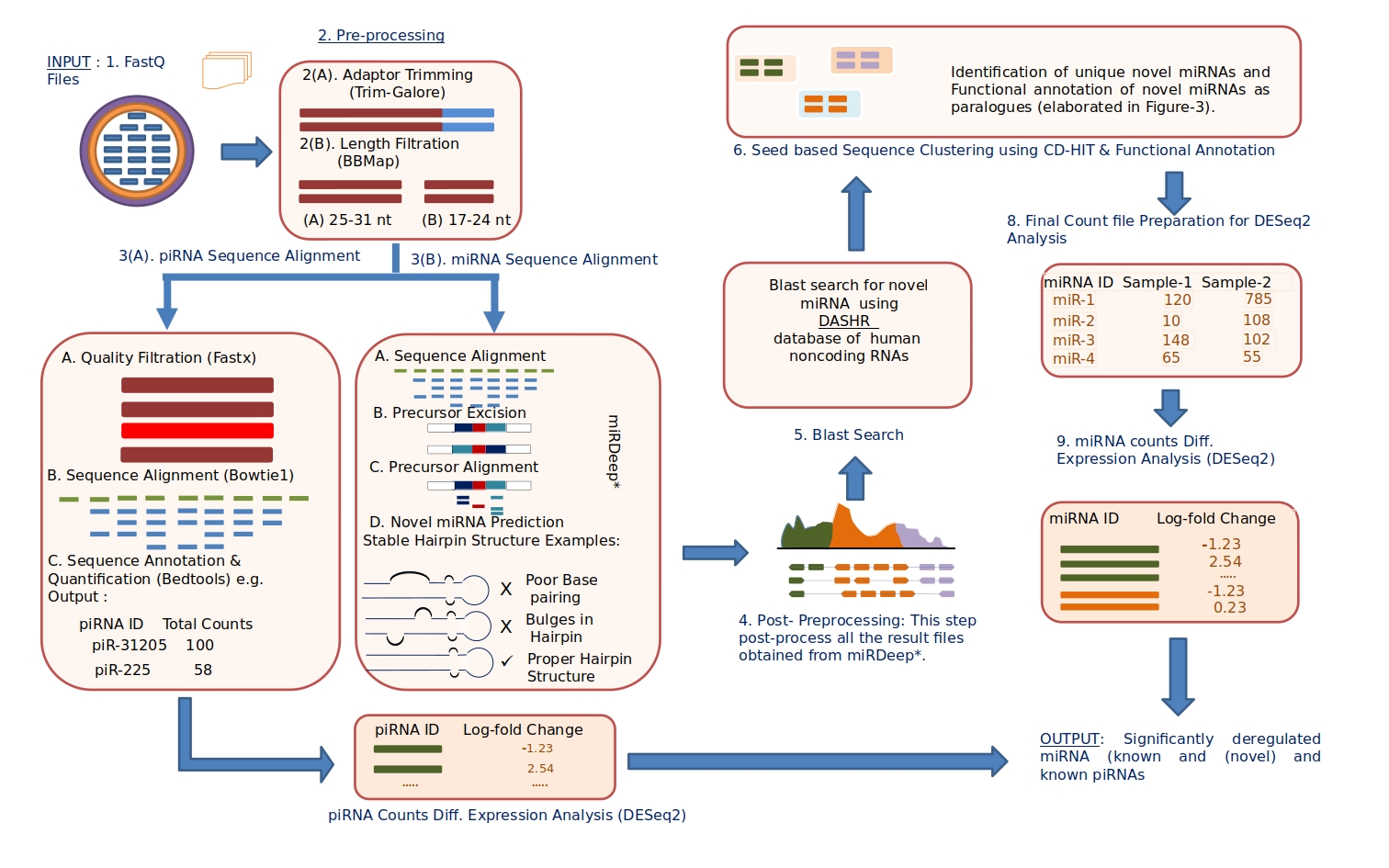
<p><img src="https://raw.githubusercontent.com/vivekruhela/miRPipe/main/Figures/R1_miRPIpe_final.jpg" alt="Published miRPipe workflow" /></p>

<p><em>Figure: miRPipe workflow supplied in the project repository. See the <a href="https://doi.org/10.3389/fbinf.2022.842051">peer-reviewed article</a> for the formal method description.</em></p>

<h3 id="who-should-use-this-guide">Who should use this guide?</h3>

<table>
  <thead>
    <tr>
      <th>Reader</th>
      <th>Recommended sections</th>
    </tr>
  </thead>
  <tbody>
    <tr>
      <td>First-time small-RNA analyst</td>
      <td>Start here, complete workflow, beginner quick start, inputs and outputs, troubleshooting</td>
    </tr>
    <tr>
      <td>Bioinformatician</td>
      <td>Advanced-user guide, limitations, comparison, reproducibility checklist</td>
    </tr>
    <tr>
      <td>Experimental biologist</td>
      <td>Start here, scientific significance, applications, outputs</td>
    </tr>
    <tr>
      <td>Reviewer or methods developer</td>
      <td>Published benchmark, limitations, comparison, reproducibility checklist</td>
    </tr>
  </tbody>
</table>

<h2 id="why-small-rna-analysis-is-difficult">Why small-RNA analysis is difficult</h2>

<p>Small RNAs are short, abundant, and often highly similar. A few nucleotides can determine whether two reads represent the same molecule, an isomiR, a paralogue, a sequencing artifact, or a different RNA class. Reads may also map to more than one genomic locus.</p>

<p>The following concepts are central to miRPipe:</p>

<table>
  <thead>
    <tr>
      <th>Term</th>
      <th>Beginner explanation</th>
      <th>Why it matters</th>
    </tr>
  </thead>
  <tbody>
    <tr>
      <td>miRNA</td>
      <td>A short regulatory RNA, commonly around 17–24 nucleotides in this workflow</td>
      <td>Its sequence and abundance can reflect gene-regulatory activity</td>
    </tr>
    <tr>
      <td>piRNA</td>
      <td>A class of small RNA commonly analyzed at longer lengths than miRNAs</td>
      <td>It requires different filtering, mapping, and annotation rules</td>
    </tr>
    <tr>
      <td>Seed region</td>
      <td>A short part of a mature miRNA that contributes strongly to target recognition</td>
      <td>Identical seeds may imply related regulatory behavior</td>
    </tr>
    <tr>
      <td>xseed region</td>
      <td>The portion outside the defined seed segment in the miRPipe method</td>
      <td>It helps distinguish otherwise similar candidates</td>
    </tr>
    <tr>
      <td>Paralogues</td>
      <td>Related miRNAs that may share a seed sequence but originate from different loci</td>
      <td>Collapsing or separating them changes interpretation and counts</td>
    </tr>
    <tr>
      <td>Reverse complement</td>
      <td>The complementary sequence written in the opposite orientation</td>
      <td>Some aligners can map it but fail to assign the expected known-miRNA label</td>
    </tr>
    <tr>
      <td>Ground truth</td>
      <td>The known identity of each simulated read</td>
      <td>It allows true positives, false positives, and false negatives to be measured</td>
    </tr>
  </tbody>
</table>

<p>miRPipe addresses these issues by combining alignment, database searches, sequence clustering, genomic-position checks, count aggregation, and statistical analysis.</p>

<h2 id="the-complete-workflow">The complete workflow</h2>

<pre><code class="language-mermaid">flowchart TD
    A["FASTQ files + sample sheet"] --&gt; B["QC and adapter trimming"]
    B --&gt; C{"Read length"}
    C --&gt;|"17–24 nt"| D["miRDeep* miRNA branch"]
    C --&gt;|"25–31 nt intended"| E["Bowtie + piRNAdb branch"]
    D --&gt; F["DASHR re-annotation"]
    F --&gt; G["Seed/xseed clustering"]
    E --&gt; H["piRNA count matrix"]
    G --&gt; I["miRNA count matrix"]
    H --&gt; J["DESeq2"]
    I --&gt; J
    J --&gt; K["Annotated and differential-expression outputs"]
</code></pre>

<h3 id="stage-by-stage-explanation">Stage-by-stage explanation</h3>

<table>
  <thead>
    <tr>
      <th>Stage</th>
      <th>What happens</th>
      <th>Main component</th>
      <th>Main output</th>
      <th>Important check</th>
    </tr>
  </thead>
  <tbody>
    <tr>
      <td>1. Input</td>
      <td>Raw reads and sample metadata are collected</td>
      <td>Jupyter/Python</td>
      <td>Valid input set</td>
      <td>Sample names and filenames must match exactly</td>
    </tr>
    <tr>
      <td>2. Initial QC</td>
      <td>Per-sample and combined quality reports are produced</td>
      <td>FastQC, MultiQC</td>
      <td>QC reports</td>
      <td>Confirm adapter sequence, read quality, and length distribution</td>
    </tr>
    <tr>
      <td>3. Adapter trimming</td>
      <td>Library adapters are removed</td>
      <td>Trim Galore</td>
      <td>Trimmed FASTQ files</td>
      <td>A wrong adapter can destroy signal or retain contamination</td>
    </tr>
    <tr>
      <td>4. Length and quality split</td>
      <td>Reads are assigned to miRNA, piRNA, or rejected-length groups</td>
      <td>BBDuk; FASTX quality filter</td>
      <td>Length-specific FASTQ files</td>
      <td>The paper and current script differ at the 24-nt boundary; see the advanced notes</td>
    </tr>
    <tr>
      <td>5A. miRNA alignment</td>
      <td>Reads are aligned and classified as known or candidate novel miRNAs</td>
      <td>miRDeep* over Bowtie</td>
      <td>Per-sample miRNA results</td>
      <td>Reference build and miRBase version must agree</td>
    </tr>
    <tr>
      <td>5B. piRNA alignment</td>
      <td>Quality-filtered reads are mapped to the human genome and annotated</td>
      <td>Bowtie, SAMtools, BEDTools, piRNAdb</td>
      <td>Per-sample piRNA counts</td>
      <td>The supplied branch uses exact mapping and disables reverse-complement alignment</td>
    </tr>
    <tr>
      <td>6. Count aggregation</td>
      <td>Results from all samples are merged</td>
      <td>Python/pandas</td>
      <td>Cohort-wide raw counts</td>
      <td>Confirm that each count column belongs to the correct sample</td>
    </tr>
    <tr>
      <td>7. Re-annotation</td>
      <td>Candidate novel sequences are checked against DASHR, including reverse complements</td>
      <td>DASHR search</td>
      <td>Corrected known/novel labels</td>
      <td>This browser-driven step is sensitive to external website and browser changes</td>
    </tr>
    <tr>
      <td>8. Seed-based clustering</td>
      <td>Candidates are compared by seed, xseed sequence, and genomic location</td>
      <td>CD-HIT plus custom Python logic</td>
      <td>Unique candidates and paralogue groups</td>
      <td>Review merged counts and locus assignments before biological interpretation</td>
    </tr>
    <tr>
      <td>9. Differential expression</td>
      <td>Counts are normalized and groups are compared</td>
      <td>DESeq2</td>
      <td>Statistics and significant-feature lists</td>
      <td>The supplied script expects <code class="language-plaintext highlighter-rouge">treated</code> and <code class="language-plaintext highlighter-rouge">untreated</code> and models <code class="language-plaintext highlighter-rouge">~ condition</code> only</td>
    </tr>
    <tr>
      <td>10. Naming and export</td>
      <td>Putative novel candidates are checked against Rfam and exported</td>
      <td>Infernal/Rfam plus Python</td>
      <td>Final annotated tables</td>
      <td>Novel names ending in <code class="language-plaintext highlighter-rouge">*</code> are putative labels, not official miRBase registrations</td>
    </tr>
  </tbody>
</table>

<h2 id="beginner-quick-start">Beginner quick start</h2>

<h3 id="1-confirm-that-your-experiment-is-appropriate">1. Confirm that your experiment is appropriate</h3>

<p>The published implementation is most directly suited to <strong>human, single-end small-RNA FASTQ data</strong>. For differential expression, prepare biological replicates in two groups. Do not treat technical replicates as independent biological samples.</p>

<p>Before running the pipeline, record:</p>

<ul>
  <li>library-preparation kit and adapter sequence;</li>
  <li>sequencing orientation and quality encoding;</li>
  <li>reference genome build (<code class="language-plaintext highlighter-rouge">hg19</code> or <code class="language-plaintext highlighter-rouge">hg38</code>);</li>
  <li>miRNA annotation version;</li>
  <li>biological condition for each sample; and</li>
  <li>any known batch, sex, age, or clinical covariates.</li>
</ul>

<p>The supplied DESeq2 script does not model those additional covariates. If they matter, export the count matrix and run a customized DESeq2 design outside the notebook.</p>

<h3 id="2-prepare-the-data-directory">2. Prepare the data directory</h3>

<p>Place the FASTQ files and <code class="language-plaintext highlighter-rouge">sample_list.csv</code> in one directory. A minimal sample sheet is:</p>

<pre><code class="language-csv">sample,file,condition
Sample_A,Sample_A.fastq.gz,treated
Sample_B,Sample_B.fastq.gz,treated
Sample_C,Sample_C.fastq.gz,untreated
Sample_D,Sample_D.fastq.gz,untreated
</code></pre>

<p>For the current notebook and R script:</p>

<ul>
  <li>use the exact column names shown above;</li>
  <li>keep sample IDs unique;</li>
  <li>use the exact group values <code class="language-plaintext highlighter-rouge">treated</code> and <code class="language-plaintext highlighter-rouge">untreated</code>;</li>
  <li>verify that every listed file exists; and</li>
  <li>sort sample rows alphanumerically, because the published implementation relies on the sample order matching the final count-matrix columns.</li>
</ul>

<p>Recommended layout:</p>

<div class="language-text highlighter-rouge"><div class="highlight"><pre class="highlight"><code>mirpipe-run/
└── data/
    ├── sample_list.csv
    ├── Sample_A.fastq.gz
    ├── Sample_B.fastq.gz
    ├── Sample_C.fastq.gz
    └── Sample_D.fastq.gz
</code></pre></div></div>

<h3 id="3-pull-and-run-the-docker-image">3. Pull and run the Docker image</h3>

<div class="language-bash highlighter-rouge"><div class="highlight"><pre class="highlight"><code>docker pull docker.io/vivekruhela/mirpipe

docker run <span class="nt">--rm</span> <span class="se">\</span>
  <span class="nt">-p</span> 127.0.0.1:8880:8888 <span class="se">\</span>
  <span class="nt">-e</span> <span class="nv">PASSWORD</span><span class="o">=</span><span class="s1">'replace-with-a-strong-local-password'</span> <span class="se">\</span>
  <span class="nt">-e</span> <span class="nv">USE_HTTP</span><span class="o">=</span>1 <span class="se">\</span>
  <span class="nt">-v</span> <span class="s2">"</span><span class="si">$(</span><span class="nb">pwd</span><span class="si">)</span><span class="s2">/data:/miRPipe/data"</span> <span class="se">\</span>
  docker.io/vivekruhela/mirpipe
</code></pre></div></div>

<p>Open <a href="http://localhost:8880/mirpipe">http://localhost:8880/mirpipe</a> and enter the password chosen in the command. Open the repository’s actual pipeline notebook, <strong><code class="language-plaintext highlighter-rouge">mirpipe_pipeline.ipynb</code></strong>.</p>

<p>The <code class="language-plaintext highlighter-rouge">127.0.0.1</code> binding keeps the unencrypted Jupyter service local to the computer. On a remote Linux server, use an SSH tunnel rather than exposing port 8880 publicly:</p>

<div class="language-bash highlighter-rouge"><div class="highlight"><pre class="highlight"><code>ssh <span class="nt">-L</span> 8880:127.0.0.1:8880 username@server.example.edu
</code></pre></div></div>

<p>Then open the same localhost address on your own computer.</p>

<blockquote>
  <p>Security note: never reuse an institutional, GitHub, Docker Hub, or email password as the notebook password. Do not expose this HTTP notebook directly to the internet.</p>
</blockquote>

<h3 id="4-run-the-notebook-carefully">4. Run the notebook carefully</h3>

<p>Run one section at a time and inspect its output before continuing.</p>

<ol>
  <li>Confirm the printed home, data, tools, and reference directories.</li>
  <li>Review FastQC/MultiQC reports.</li>
  <li>Select the correct adapter option.</li>
  <li>Select a compatible genome-build and miRBase combination.</li>
  <li>Run the miRNA and/or piRNA branch.</li>
  <li>Check the number of known and candidate novel features.</li>
  <li>Review re-annotation and seed-clustering results.</li>
  <li>Confirm the count-matrix column order against <code class="language-plaintext highlighter-rouge">sample_list.csv</code>.</li>
  <li>Run DESeq2 only after those checks pass.</li>
  <li>Copy final results and all run metadata to a permanent project directory.</li>
</ol>

<h2 id="inputs-and-outputs">Inputs and outputs</h2>

<h3 id="required-inputs">Required inputs</h3>

<table>
  <thead>
    <tr>
      <th>Input</th>
      <th style="text-align: right">Required?</th>
      <th>Description</th>
    </tr>
  </thead>
  <tbody>
    <tr>
      <td>FASTQ/FASTQ.GZ</td>
      <td style="text-align: right">Yes</td>
      <td>Raw small-RNA sequencing reads</td>
    </tr>
    <tr>
      <td><code class="language-plaintext highlighter-rouge">sample_list.csv</code></td>
      <td style="text-align: right">Required for cohort/DE analysis</td>
      <td>Sample, filename, and condition mapping</td>
    </tr>
    <tr>
      <td>Adapter sequence</td>
      <td style="text-align: right">Yes, explicit or default</td>
      <td>Must match the library-preparation protocol</td>
    </tr>
    <tr>
      <td>Reference genome</td>
      <td style="text-align: right">Yes</td>
      <td>Human <code class="language-plaintext highlighter-rouge">hg19</code> or <code class="language-plaintext highlighter-rouge">hg38</code> in the published workflow</td>
    </tr>
    <tr>
      <td>miRNA/piRNA annotations</td>
      <td style="text-align: right">Yes</td>
      <td>miRBase and piRNAdb resources matching the chosen build</td>
    </tr>
  </tbody>
</table>

<h3 id="five-final-output-files-documented-in-the-repository">Five final output files documented in the repository</h3>

<table>
  <thead>
    <tr>
      <th>File</th>
      <th>Meaning</th>
      <th>Typical downstream use</th>
    </tr>
  </thead>
  <tbody>
    <tr>
      <td><code class="language-plaintext highlighter-rouge">final_diff_exp_miRNAs.csv</code></td>
      <td>Significant known/novel miRNAs with effect and annotation fields</td>
      <td>Candidate prioritization and reporting</td>
    </tr>
    <tr>
      <td><code class="language-plaintext highlighter-rouge">diff_exp_miRNAs_expression_counts.csv</code></td>
      <td>Counts for significant miRNAs</td>
      <td>Heatmaps and sample-level inspection</td>
    </tr>
    <tr>
      <td><code class="language-plaintext highlighter-rouge">miRNA_expression_counts.csv</code></td>
      <td>Cohort miRNA raw-count matrix</td>
      <td>Customized DESeq2/edgeR analysis</td>
    </tr>
    <tr>
      <td><code class="language-plaintext highlighter-rouge">piRNA_raw_counts.csv</code></td>
      <td>Cohort piRNA raw-count matrix</td>
      <td>Customized piRNA analysis</td>
    </tr>
    <tr>
      <td><code class="language-plaintext highlighter-rouge">significantly_DE_piRNA.csv</code></td>
      <td>Significant piRNA identifiers</td>
      <td>Candidate follow-up</td>
    </tr>
  </tbody>
</table>

<p>Also retain the QC reports, complete DESeq2 result tables, normalized counts, software versions, logs, and intermediate annotation tables. A significant-only table is insufficient for reproducible review.</p>

<p><img src="https://raw.githubusercontent.com/vivekruhela/miRPipe/main/Figures/Sample_list.png" alt="Example sample sheet" /></p>

<h2 id="advanced-user-guide">Advanced-user guide</h2>

<h3 id="read-length-boundary">Read-length boundary</h3>

<p>The paper describes 17–24 nt reads for miRNA analysis and 25–31 nt reads for piRNA analysis. The current <code class="language-plaintext highlighter-rouge">scripts/fastq_split.sh</code>, however, sets <code class="language-plaintext highlighter-rouge">minlength=24</code> and <code class="language-plaintext highlighter-rouge">maxlength=31</code> for the piRNA branch. That creates a 24-nt overlap between the two branches.</p>

<p>Before a new study, decide whether to reproduce the published intention or the repository implementation. Record the decision and benchmark it because a one-nucleotide boundary can change RNA-class assignment.</p>

<h3 id="pirna-mapping-behavior">piRNA mapping behavior</h3>

<p>The supplied piRNA script uses Bowtie with exact matching (<code class="language-plaintext highlighter-rouge">-v 0</code>), disables reverse-complement alignment (<code class="language-plaintext highlighter-rouge">--norc</code>), and quantifies overlap with piRNAdb annotations. These choices are stringent. They can reduce false-positive mappings but can also miss legitimate reads containing sequencing errors, biological variation, or opposite-strand mappings.</p>

<p>For a new production study, document:</p>

<ul>
  <li>unique versus multi-mapping policy;</li>
  <li>allowed mismatches;</li>
  <li>strand rule;</li>
  <li>annotation database and release;</li>
  <li>genome build; and</li>
  <li>how overlapping annotations are counted.</li>
</ul>

<h3 id="mirna-alignment-and-re-annotation">miRNA alignment and re-annotation</h3>

<p>miRDeep* performs the initial known/novel miRNA classification. miRPipe then checks candidate novel sequences against DASHR. If a sequence or its reverse complement matches a known miRNA at a compatible locus, its label and counts can be reassigned.</p>

<p>This is one of the method’s distinctive ideas, but the notebook automates a public website through an older Firefox/Splinter/geckodriver setup. For stable modern operation, replace browser automation with a versioned, locally downloadable annotation resource or a documented API if licensing and availability permit.</p>

<h3 id="seedxseed-clustering-logic">Seed/xseed clustering logic</h3>

<p>The published method uses the following concepts:</p>

<ol>
  <li>Group sequences with identical seed regions.</li>
  <li>Compare the sequence outside the seed.</li>
  <li>Treat candidates with identical seed, no more than two xseed changes, and genomic positions within two nucleotides as one novel miRNA; merge their counts.</li>
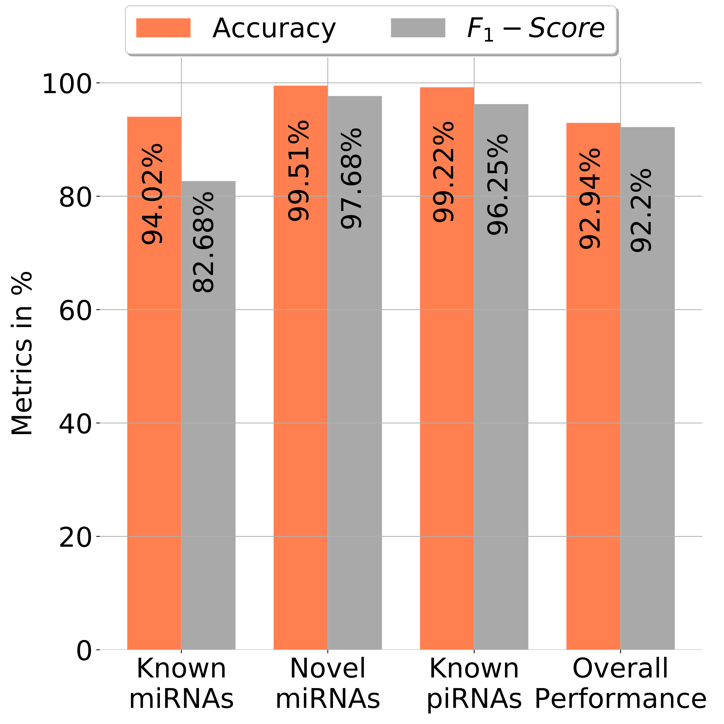
  <li>Treat identical-seed candidates at different loci as paralogue candidates.</li>
  <li>Associate a novel candidate with a known family when it shares the known miRNA seed but maps to a different locus.</li>
</ol>

<pre><code class="language-mermaid">flowchart TD
    A["Candidate sequences"] --&gt; B{"Identical seed?"}
    B --&gt;|No| C["Separate candidates"]
    B --&gt;|Yes| D{"xseed difference ≤2 nt?"}
    D --&gt;|No| C
    D --&gt;|Yes| E{"Genomic positions within 2 nt?"}
    E --&gt;|Yes| F["Merge as one candidate"]
    E --&gt;|No| G["Report paralogue relationship"]
</code></pre>

<p>These operational rules are useful for reproducibility, but “same seed” does not by itself prove identical biological function. Target context, arm selection, expression, localization, and experimental validation still matter.</p>

<h3 id="differential-expression-model">Differential-expression model</h3>

<p>The supplied <code class="language-plaintext highlighter-rouge">scripts/norm_diff_exp.R</code> uses:</p>

<div class="language-r highlighter-rouge"><div class="highlight"><pre class="highlight"><code><span class="n">design</span><span class="w"> </span><span class="o">=</span><span class="w"> </span><span class="o">~</span><span class="w"> </span><span class="n">condition</span><span class="w">
</span><span class="n">contrast</span><span class="w"> </span><span class="o">=</span><span class="w"> </span><span class="nf">c</span><span class="p">(</span><span class="s2">"condition"</span><span class="p">,</span><span class="w"> </span><span class="s2">"treated"</span><span class="p">,</span><span class="w"> </span><span class="s2">"untreated"</span><span class="p">)</span><span class="w">
</span></code></pre></div></div>

<p>It applies the Benjamini–Hochberg procedure and selects features with adjusted p-value ≤ 0.05. The script does not include batch, age, sex, paired design, repeated measures, surrogate variables, or fold-change shrinkage.</p>

<p>For complex studies, use the exported raw-count matrix with an appropriate design, for example:</p>

<div class="language-r highlighter-rouge"><div class="highlight"><pre class="highlight"><code><span class="n">design</span><span class="w"> </span><span class="o">=</span><span class="w"> </span><span class="o">~</span><span class="w"> </span><span class="n">batch</span><span class="w"> </span><span class="o">+</span><span class="w"> </span><span class="n">sex</span><span class="w"> </span><span class="o">+</span><span class="w"> </span><span class="n">age</span><span class="w"> </span><span class="o">+</span><span class="w"> </span><span class="n">condition</span><span class="w">
</span></code></pre></div></div>

<p>The exact model must follow the experimental design; the example is not universally appropriate. Also consider low-count prefiltering, independent filtering, effect-size thresholds, unwanted-variation diagnostics, and shrinkage of log2 fold changes.</p>

<h3 id="scaling-to-cohorts-and-hpc">Scaling to cohorts and HPC</h3>

<p>miRPipe batches samples and runs miRDeep* work in Python threads, while the piRNA branch runs concurrently. This can accelerate multi-sample processing, but resource control is implemented inside a notebook rather than through a scheduler-aware workflow engine.</p>

<p>For an HPC deployment:</p>

<ul>
  <li>run one container image identified by immutable digest;</li>
  <li>allocate memory per concurrent miRDeep* task;</li>
  <li>avoid oversubscribing CPUs inside a SLURM allocation;</li>
  <li>separate temporary and permanent storage;</li>
  <li>retain per-sample logs and exit codes;</li>
  <li>use a manifest rather than depending on directory glob order; and</li>
  <li>consider refactoring stages into Nextflow, Snakemake, or CWL while preserving miRPipe’s re-annotation and clustering logic.</li>
</ul>

<h3 id="minimum-qc-report-for-a-publication">Minimum QC report for a publication</h3>

<p>Report at least:</p>

<ul>
  <li>samples received, excluded, and analyzed;</li>
  <li>reads before and after adapter/quality filtering;</li>
  <li>read-length distribution;</li>
  <li>fraction assigned to miRNA, piRNA, other small RNA, and unmapped;</li>
  <li>mapping-rate and multi-mapping distribution;</li>
  <li>known versus candidate novel counts;</li>
  <li>number of candidates re-annotated through DASHR;</li>
  <li>number of clusters merged and paralogue groups reported;</li>
  <li>PCA/sample-distance plots from final counts;</li>
  <li>DE model, contrasts, covariates, multiple-testing rule, and effect-size rule; and</li>
  <li>exact software, container, reference, and database versions.</li>
</ul>

<h2 id="scientific-significance">Scientific significance</h2>

<h3 id="methodological-significance">Methodological significance</h3>

<p>miRPipe combines tasks that were often handled separately: known and novel miRNA discovery, piRNA quantification, reverse-complement rescue, seed-based candidate reconciliation, cohort count-matrix construction, and differential expression. Its companion simulator, miRSim, provides ground truth for measuring false positives and false negatives.</p>

<h3 id="biological-significance">Biological significance</h3>

<p>Small RNAs regulate gene expression and may reflect disease mechanisms, cell states, or treatment responses. Reliable classification matters because an incorrect label or duplicated count can redirect downstream target prediction, enrichment, biomarker selection, and experimental validation.</p>

<h3 id="reproducibility-significance">Reproducibility significance</h3>

<p>Containerization and a notebook lower the installation barrier and make the intended analysis visible. The design was especially valuable for users who needed an integrated workflow in 2022. A modern refresh should retain that accessibility while adding immutable images, command-line configuration, automated tests, and scheduler-aware execution.</p>

<h2 id="applications">Applications</h2>

<p>miRPipe can support:</p>

<ul>
  <li>exploratory small-RNA profiling in cancer and other diseases;</li>
  <li>identification of known and candidate novel miRNAs;</li>
  <li>cohort-level differential-expression analysis;</li>
  <li>piRNA quantification from compatible small-RNA libraries;</li>
  <li>paralogue-aware review of miRNA candidates;</li>
  <li>re-evaluation of candidates affected by reverse-complement labeling;</li>
  <li>benchmarking of small-RNA pipelines using miRSim ground truth;</li>
  <li>method development and sensitivity analysis; and</li>
  <li>non-human analyses after validated replacement of the genome and annotation resources.</li>
</ul>

<p>It should <strong>not</strong> be presented as a clinical diagnostic system without independent analytical validation, biological validation, version-controlled references, quality-management procedures, and appropriate regulatory review.</p>

<h2 id="published-benchmark">Published benchmark</h2>

<p>The 2022 article compared miRPipe with seven pipelines using miRSim synthetic data at 50,000, 100,000, and 1,000,000 reads. The following values reproduce the averages reported in Table 2 of the paper.</p>

<table>
  <thead>
    <tr>
      <th>Pipeline</th>
      <th style="text-align: right">Known miRNA accuracy</th>
      <th style="text-align: right">Known miRNA F1</th>
      <th style="text-align: right">Novel miRNA accuracy</th>
      <th style="text-align: right">Novel miRNA F1</th>
      <th style="text-align: right">Known piRNA accuracy</th>
      <th style="text-align: right">Known piRNA F1</th>
    </tr>
  </thead>
  <tbody>
    <tr>
      <td>miRDeep2</td>
      <td style="text-align: right">94.74%</td>
      <td style="text-align: right">85.66%</td>
      <td style="text-align: right">97.33%</td>
      <td style="text-align: right">85.27%</td>
      <td style="text-align: right">—</td>
      <td style="text-align: right">—</td>
    </tr>
    <tr>
      <td>miRDeep*</td>
      <td style="text-align: right">95.67%</td>
      <td style="text-align: right">88.06%</td>
      <td style="text-align: right">99.04%</td>
      <td style="text-align: right">95.47%</td>
      <td style="text-align: right">—</td>
      <td style="text-align: right">—</td>
    </tr>
    <tr>
      <td>mirPRo</td>
      <td style="text-align: right">78.73%</td>
      <td style="text-align: right">1.45%</td>
      <td style="text-align: right">93.04%</td>
      <td style="text-align: right">60.93%</td>
      <td style="text-align: right">—</td>
      <td style="text-align: right">—</td>
    </tr>
    <tr>
      <td>mirnovo</td>
      <td style="text-align: right">87.59%</td>
      <td style="text-align: right">60.61%</td>
      <td style="text-align: right">91.78%</td>
      <td style="text-align: right">41.95%</td>
      <td style="text-align: right">—</td>
      <td style="text-align: right">—</td>
    </tr>
    <tr>
      <td>miRge2.0</td>
      <td style="text-align: right">82.56%</td>
      <td style="text-align: right">25.90%</td>
      <td style="text-align: right">0.00%</td>
      <td style="text-align: right">0.00%</td>
      <td style="text-align: right">—</td>
      <td style="text-align: right">—</td>
    </tr>
    <tr>
      <td>sRNAbench</td>
      <td style="text-align: right">89.18%</td>
      <td style="text-align: right">67.93%</td>
      <td style="text-align: right">0.00%</td>
      <td style="text-align: right">0.00%</td>
      <td style="text-align: right">74.25%</td>
      <td style="text-align: right">4.34%</td>
    </tr>
    <tr>
      <td>MiR&amp;moRe2</td>
      <td style="text-align: right">91.07%</td>
      <td style="text-align: right">74.05%</td>
      <td style="text-align: right">92.52%</td>
      <td style="text-align: right">46.76%</td>
      <td style="text-align: right">—</td>
      <td style="text-align: right">—</td>
    </tr>
    <tr>
      <td><strong>miRPipe</strong></td>
      <td style="text-align: right"><strong>96.58%</strong></td>
      <td style="text-align: right"><strong>89.95%</strong></td>
      <td style="text-align: right"><strong>99.55%</strong></td>
      <td style="text-align: right"><strong>97.55%</strong></td>
      <td style="text-align: right"><strong>98.91%</strong></td>
      <td style="text-align: right"><strong>94.35%</strong></td>
    </tr>
  </tbody>
</table>

<p>The reported overall average was approximately 95.22% accuracy and 94.17% F1 across RNA types and depths. The abstract reports 95.23% for accuracy, a small rounding/reporting difference.</p>

<table>
  <tr>
    <th>50K reads</th>
    <th>0.1M reads</th>
    <th>1M reads</th>
  </tr>
  <tr>
    <td><img alt="Benchmark at 50K reads" src="https://raw.githubusercontent.com/vivekruhela/miRPipe/main/Figures/50K_overall.png" /></td>
    <td><img alt="Benchmark at 0.1M reads" src="https://raw.githubusercontent.com/vivekruhela/miRPipe/main/Figures/1L_overall.png" /></td>
    <td><img alt="Benchmark at 1M reads" src="https://raw.githubusercontent.com/vivekruhela/miRPipe/main/Figures/10L_overall.png" /></td>
  </tr>
</table>

<h2 id="comparison-with-other-pipelines">Comparison with other pipelines</h2>

<p>The table below is a <strong>capability-oriented current-use guide</strong>, not a new head-to-head performance benchmark.</p>

<table>
  <thead>
    <tr>
      <th>Tool/workflow</th>
      <th>Strong use case</th>
      <th>Relevant capabilities</th>
      <th>Main trade-off relative to miRPipe</th>
    </tr>
  </thead>
  <tbody>
    <tr>
      <td><strong>miRPipe</strong></td>
      <td>Reproducing the published method; joint miRNA/piRNA analysis with seed/paralogue logic</td>
      <td>Known/novel miRNA, annotated piRNA, reverse-complement review, DESeq2, Docker/Jupyter</td>
      <td>Older dependencies and brittle external searches; limited automation/testing in the current repository</td>
    </tr>
    <tr>
      <td><strong>miRDeep2</strong></td>
      <td>Classic known and novel miRNA discovery</td>
      <td>Mature/precursor evidence, novel-miRNA scoring, expression profiling</td>
      <td>Does not provide miRPipe’s integrated piRNA, reverse-complement, seed-clustering, and cohort-DE wrapper</td>
    </tr>
    <tr>
      <td><strong>miRge3.0</strong></td>
      <td>Feature-rich miRNA and tRF profiling</td>
      <td>miRNA, isomiR, novel miRNA, tRF, UMI processing, A-to-I editing, CLI/GUI</td>
      <td>Different biological scope; not a direct replacement for miRPipe’s dedicated piRNA branch or clustering rules</td>
    </tr>
    <tr>
      <td><strong>sRNAbench / sRNAtoolbox</strong></td>
      <td>Broad small-RNA profiling and accessible web/Docker workflows</td>
      <td>miRNA and other sncRNAs, differential expression, unmapped-read analysis, target analysis; model and non-model organisms</td>
      <td>Uses its own annotation and prediction framework; does not reproduce miRPipe’s exact candidate reconciliation</td>
    </tr>
    <tr>
      <td><strong>nf-core/smrnaseq</strong></td>
      <td>Reproducible production analysis on HPC/cloud</td>
      <td>Nextflow, containers per process, automated tests, FastQC/MultiQC, miRTrace, mirtop/isomiR, miRDeep2, edgeR</td>
      <td>Stronger workflow engineering, but no equivalent dedicated miRPipe seed/paralogue and piRNAdb branch</td>
    </tr>
  </tbody>
</table>

<h3 id="practical-selection-guide">Practical selection guide</h3>

<ul>
  <li>Choose <strong>miRPipe</strong> when the scientific question specifically needs the published reverse-complement, seed/xseed, paralogue, and joint miRNA/piRNA logic.</li>
  <li>Choose <strong>nf-core/smrnaseq</strong> when production-grade portability, automated testing, provenance, HPC execution, and broad QC are the primary needs.</li>
  <li>Choose <strong>miRge3.0</strong> when UMI, isomiR, tRF, or A-to-I editing analysis is central.</li>
  <li>Choose <strong>sRNAtoolbox/sRNAbench</strong> for broad small-RNA profiling, web access, Docker deployment, or non-model organisms.</li>
  <li>Choose <strong>miRDeep2</strong> for a focused and widely recognized known/novel miRNA discovery workflow.</li>
</ul>

<p>For a new methods paper, benchmark multiple tools under the same inputs, reference versions, compute limits, parameter-tuning policy, and independent ground truth.</p>

<h2 id="troubleshooting">Troubleshooting</h2>

<table>
  <thead>
    <tr>
      <th>Symptom</th>
      <th>Likely cause</th>
      <th>What to check</th>
    </tr>
  </thead>
  <tbody>
    <tr>
      <td>Jupyter page does not open</td>
      <td>Container stopped, port conflict, or incorrect URL</td>
      <td>Run <code class="language-plaintext highlighter-rouge">docker ps</code>; confirm port <code class="language-plaintext highlighter-rouge">8880</code>; use <code class="language-plaintext highlighter-rouge">/mirpipe</code> in the URL</td>
    </tr>
    <tr>
      <td>FASTQ files are not visible</td>
      <td>Incorrect bind-mount source or destination</td>
      <td>Mount the host data directory to <code class="language-plaintext highlighter-rouge">/miRPipe/data</code></td>
    </tr>
    <tr>
      <td>Adapter-trimming results are empty or poor</td>
      <td>Wrong adapter or incompatible filename handling</td>
      <td>Confirm kit adapter; inspect Trim Galore log; test one sample manually</td>
    </tr>
    <tr>
      <td>No miRNAs are detected</td>
      <td>Wrong build/database, poor small-RNA library, or overly strict filtering</td>
      <td>Check read lengths, mapping rate, reference selection, and FastQC/MultiQC</td>
    </tr>
    <tr>
      <td>Unexpected overlap between RNA classes</td>
      <td>24-nt boundary discrepancy</td>
      <td>Inspect <code class="language-plaintext highlighter-rouge">scripts/fastq_split.sh</code>; document and test the chosen boundary</td>
    </tr>
    <tr>
      <td>DASHR step fails</td>
      <td>Website, Firefox, Splinter, or geckodriver incompatibility</td>
      <td>Preserve candidates; perform a documented local re-annotation alternative rather than silently skipping the step</td>
    </tr>
    <tr>
      <td>DESeq2 contrast error</td>
      <td>Group names differ from hard-coded values</td>
      <td>Use exactly <code class="language-plaintext highlighter-rouge">treated</code> and <code class="language-plaintext highlighter-rouge">untreated</code>, or edit the R contrast deliberately</td>
    </tr>
    <tr>
      <td>Sample labels do not match count columns</td>
      <td>Ordering dependency or inconsistent filenames</td>
      <td>Sort and compare <code class="language-plaintext highlighter-rouge">sample_list.csv</code> with the final matrix before DESeq2</td>
    </tr>
    <tr>
      <td>No significant features</td>
      <td>Low power, weak effect, high dispersion, or multiple-testing burden</td>
      <td>Inspect all results, sample distances, counts, effect sizes, and study design; do not relax FDR only to obtain hits</td>
    </tr>
    <tr>
      <td>Non-human analysis fails</td>
      <td>Human-specific reference paths and annotations</td>
      <td>Build and validate species-specific indices and annotation resources throughout all branches</td>
    </tr>
  </tbody>
</table>

<h2 id="citation">Citation</h2>

<p>If miRPipe is used, cite:</p>

<blockquote>
  <p>Ruhela V, Gupta A, Sriram K, Ahuja G, Kaur G, Gupta R. A Unified Computational Framework for a Robust, Reliable, and Reproducible Identification of Novel miRNAs From the RNA Sequencing Data. <em>Frontiers in Bioinformatics</em>. 2022;2:842051. <a href="https://doi.org/10.3389/fbinf.2022.842051">https://doi.org/10.3389/fbinf.2022.842051</a></p>
</blockquote>

<p>BibTeX:</p>

<div class="language-bibtex highlighter-rouge"><div class="highlight"><pre class="highlight"><code><span class="nc">@article</span><span class="p">{</span><span class="nl">ruhela2022mirpipe</span><span class="p">,</span>
  <span class="na">title</span>   <span class="p">=</span> <span class="s">{A Unified Computational Framework for a Robust, Reliable, and Reproducible Identification of Novel miRNAs From the RNA Sequencing Data}</span><span class="p">,</span>
  <span class="na">author</span>  <span class="p">=</span> <span class="s">{Ruhela, Vivek and Gupta, Anubha and Sriram, K. and Ahuja, Gaurav and Kaur, Gurvinder and Gupta, Ritu}</span><span class="p">,</span>
  <span class="na">journal</span> <span class="p">=</span> <span class="s">{Frontiers in Bioinformatics}</span><span class="p">,</span>
  <span class="na">volume</span>  <span class="p">=</span> <span class="s">{2}</span><span class="p">,</span>
  <span class="na">pages</span>   <span class="p">=</span> <span class="s">{842051}</span><span class="p">,</span>
  <span class="na">year</span>    <span class="p">=</span> <span class="s">{2022}</span><span class="p">,</span>
  <span class="na">doi</span>     <span class="p">=</span> <span class="s">{10.3389/fbinf.2022.842051}</span>
<span class="p">}</span>
</code></pre></div></div>

<h2 id="project-and-comparison-resources">Project and comparison resources</h2>

<ul>
  <li><a href="https://github.com/vivekruhela/miRPipe">miRPipe source repository</a></li>
  <li><a href="https://www.frontiersin.org/journals/bioinformatics/articles/10.3389/fbinf.2022.842051/full">miRPipe article</a></li>
  <li><a href="https://github.com/vivekruhela/miRSim">miRSim source repository</a></li>
  <li><a href="https://www.mdc-berlin.de/content/mirdeep2-documentation">miRDeep2 documentation</a></li>
  <li><a href="https://github.com/mhalushka/miRge3.0">miRge3.0 source and documentation</a></li>
  <li><a href="https://github.com/bioinfoUGR/sRNAtoolbox">sRNAtoolbox source and documentation</a></li>
  <li><a href="https://nf-co.re/smrnaseq/2.4.1/">nf-core/smrnaseq</a></li>
</ul>]]></content><author><name>Vivek Ruhela</name><email>vr2592@cumc.columbia.edu</email></author><summary type="html"><![CDATA[miRPipe: Beginner and Advanced User Guide]]></summary></entry></feed>